6
$\begingroup$

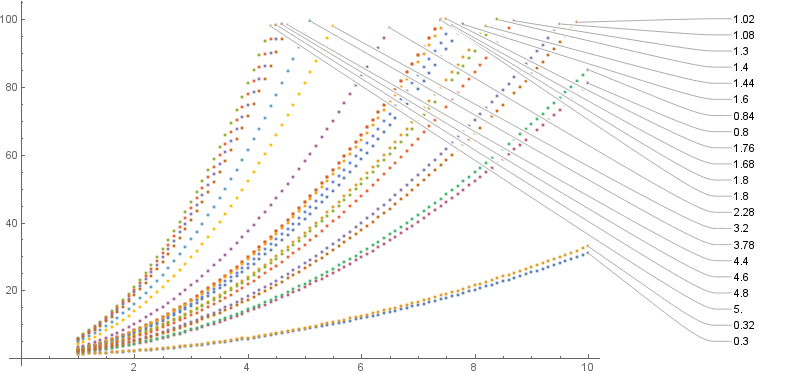
I recently updated to Mathematica 11.2, and I very much like the automatic PlotLabels feature that I discovered. However, it picks a somewhat silly ordering when the data I'm plotting cuts off at different x-locations. Say I have data that looks something like this:

slopes = Table[i Round[Abs[Sin[i]], 0.1], {i, 1, 5, 0.2}]; mydata = Table[Select[Table[{x, 1 + slope * x^2}, {x, 1, 10, 0.1}], #1[[2]] < 100 &], {slope, slopes}]; 

If I just ListPlot it, Mathematica does something smart about plot label vertical positioning which I haven't managed to recreate manually:

ListPlot[mydata, PlotLabels -> slopes, ImageSize -> Large] 

smart PlotLabels

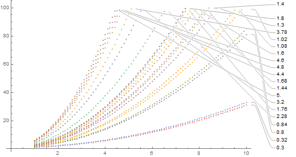
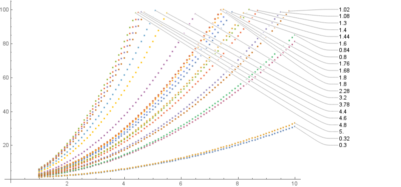
However, the ordering is all off; I want to order them by the slope, not by the y-value at the location where my data happened to cut off. So I tried using Callout instead, with a manually specified anchor position:

ListPlot[Map[Callout[#1[[1]], #1[[2]], Automatic, 5] &, Transpose[{mydata, slopes}]], ImageSize -> Large] 

This gives the horrendous-looking

bad callout

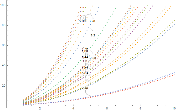
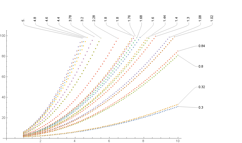
Okay, fine, I can give it a position manually. But 10 and {10, After} both give identical, very bad results:

manual x position


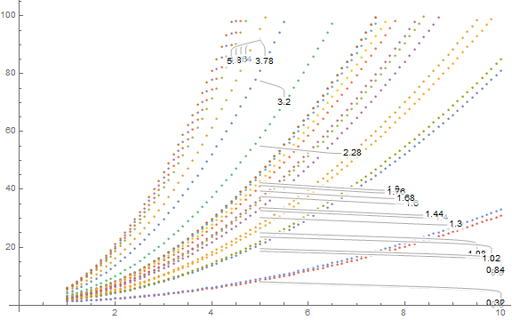
What I want, from most important to least important (but preferably all of them):

  1. the labels should not overlap and should not be cut off
  2. the labels should have a pointer to some point on the curve
  3. the labels should be in slope-order, or, more precisely, the order that the data has at a particular x-position that I specify
  4. the labels should all be along the right side of the plot, the axis should not extend past the end of the data

How can I accomplish this?

$\endgroup$
2

1 Answer 1

2
$\begingroup$

Using Callout with explicit positions for labels in the setting of PlotLabels combined with manual reordering of input data:

slopes = Sort@Table[i Round[Abs[Sin[i]], 0.1], {i, 1, 5, 0.2}]; mydata = Table[Select[Table[{x, 1 + slope * x^2}, {x, 1, 10, 0.1}], #1[[2]] <= 100 &], {slope, slopes}]; ordering ={1,2,21,20,19,18,17,16,15,14,13,11,12,3,4,10,9,8,7,6,5}; mydataordered = mydata[[ordering]]; slopesordered = slopes[[ordering]]; xpos = 12; yrange = {5, 100}; ListPlot[mydataordered, PlotLabels -> MapIndexed[Callout[#,{xpos, Rescale[#2[[1]], {1, Length@mydata}, yrange]}, mydataordered[[All,-1]][[#2[[1]]]], LeaderSize -> {{Automatic, Automatic, 0}, {30, 0 Degree}}]&, slopesordered], ImagePadding -> {{Automatic,200}, { Automatic, Automatic}}, ImageSize -> 800, PlotRangeClipping -> False] 

enter image description here

Use xpos = 11; yrange={20, 100}; to get

enter image description here

Alternatively, use

ListPlot[MapIndexed[Callout[#, slopesordered[[#2[[1]]]], {xpos, Rescale[#2[[1]], {1, Length @ mydata}, yrange]}, mydataordered[[All,-1]][[#2[[1]]]], LeaderSize -> {{Automatic, Automatic, 0}, {30, 0 Degree}}]&, mydataordered], ImagePadding -> {{Automatic, 200}, {Automatic, Automatic}}, ImageSize -> 800, PlotRangeClipping -> False] 

to get the same result as above.

Update: An alternative layout for the Callouts:

combined = Transpose[{mydata, slopes}]; {top, left} = Pick[combined, #[[1, -1, 1]] < 9.9 & /@ combined, #]&/@{True, False}; {datatop, slopestop} = Transpose[SortBy[top, #[[1,-1,1]]&]]; {dataleft, slopesleft} = Transpose[SortBy[left, #[[1,-1,-1]]&]]; dL = MapIndexed[Callout[#, slopesleft[[#2[[1]]]], {11, Rescale[#2[[1]], {1, Length @ dataleft}, {30, 90}]}, dataleft[[All,-1]][[#2[[1]]]], LeaderSize -> {{Automatic, Automatic, 0}, {10, 0 Degree}}]&, dataleft]; dT = MapIndexed[Callout[#, slopestop[[#2[[1]]]], {Rescale[#2[[1]],{1, Length @ datatop}, {1, 12}], 110}, datatop[[All, -1]][[#2[[1]]]], LeaderSize -> {{Automatic, Automatic, 0}, {10, 90 Degree}}]&, datatop]; ListPlot[Join[dL,dT], ImagePadding -> {{Automatic,200},{ Automatic, 100}}, ImageSize->800, PlotRangeClipping->False] 

enter image description here

$\endgroup$

Start asking to get answers

Find the answer to your question by asking.

Ask question

Explore related questions

See similar questions with these tags.