Currently, Mathematica treats function which has branch cuts; $\log(z)$,$\sqrt[n]{z}$, etc, by taking its principal value. This may cause a problem in Contour integration when the path of integration walks over the branch cut. This may be fixed by a wise implementation of the Integrate function. But it is still a problem in my case. That is I want to visualize how curves in a complex plane are transformed by complex functions. For example, when a point in a complex plane moves around an origin twice, I want to see the point projected by $\sqrt(z)$ move around an origin once. But Mathematica's Sqrt makes the projected point jumps discontinuously when a point walk across the branch cut as seen in the attached picture.
I think this problem can be resolved by making every complex calculation to avoid taking modulo $2\pi$ to the phase of a complex value until the last moment. So the internal representation of complex values should be polar form and there must be a wise mechanism to decide when to do modulo $2\pi$ operation to its phase.
What do you think about this idea? Is there a way to visualize the "natural path" of a projected point by complex functions that have branch cuts?
Thank you. 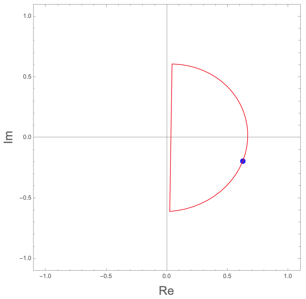
EDIT Thanks to Dominic and J. M. will be back soon, I finally achieved what I want. Thank both of you!
BranchRootsMod[exp_] := Module[ {p, f, e, k, t}, If[Head[exp] === List, t = BranchRootsMod /@ exp; , p = Position[exp, _^_Rational]; If[Length[p] > 0, f = First[p]; If[Length[f] == 0, e = exp; k = e /. _^r_Rational :> 1/r; t = Table[root[First[e], 1/k]*Exp[I ( 2 \[Pi] i)/k], {i, 0, k - 1}]; , e = Extract[exp, f]; k = e /. _^r_Rational :> 1/r; t = Table[ReplacePart[exp, f -> root[First[e], 1/k]*Exp[I ( 2 \[Pi] i)/k]], {i, 0, k - 1}]; ]; , t = exp; ]; ]; t ]; BranchRoots[exp_] := Module[{e = (FixedPoint[BranchRootsMod, exp] /. root -> Power)}, If[Head[e] === List, Flatten[e], e]]; ProjectedTrajectory[exp_, var_, traj_, range_] := Module[{w, t, trajd, wd, func, sol}, func = Simplify[First[GroebnerBasis[{w == exp}, {var, w}]]]; t = range[[1]]; trajd = D[traj, t]; wd = w'[ t] == ((-(D[func, var]/D[func, w]) trajd) /. {w -> w[t], var -> traj}); sol = First[ NDSolve[{wd, w[range[[2]]] == exp /. (var :> (traj /. t -> range[[2]]))}, w, {t, range[[2]], range[[3]]}]]; w /. sol ] tmax = 12 \[Pi]; exp = (x^(1/3) + x^(1/2) - 0.5)^(1/3); traj = ProjectedTrajectory[exp, x, Exp[I t], {t, 0, 2*tmax}]; list = Table[Through[{Re, Im}@traj[t]], {t, 0, tmax, tmax/ 100}]; Manipulate[ Module[{pts}, pts = Through[{Re, Im}@#] & /@ BranchRoots[exp] /. x -> Exp[I t]; Graphics[ { {Blue, Circle[#, 0.1]} & /@ pts, {Orange, PointSize[0.02], Point[Through[{Re, Im}@traj[t]]]}, {Orange, Line@list[[;; Floor[100*t/tmax]]]} }, PlotRange -> {{-3, 3}, {-3, 3}} ]], {t, 0, tmax} ]