Why not just using ContourPlot?
eq = -1.94178*10^24*H*Te^0.5 - (3.2*(7.33376*10^27*Te^(7/2) + 4.66533*10^24*Ti^(7/2)))/ (10^9*H) + 7.68161*10^40*H*(5.41/((10^15*E^(148/Ti))*Ti^(3/2)) + 2.00122/((10^10*E^((53.124*(1 - (-0.059357*Ti + 0.0010404*Ti^2 - (9.1653*Ti^3)/10^6)/ (1 + 0.20165*Ti + 0.0027621*Ti^2 + (9.8305*Ti^3)/10^7))^(1/3))/Ti^(1/3)))* (Ti^(2/3)*(1 - (-0.059357*Ti + 0.0010404*Ti^2 - (9.1653*Ti^3)/10^6)/ (1 + 0.20165*Ti + 0.0027621*Ti^2 + (9.8305*Ti^3)/10^7))^(5/6)))); sol = H /. Solve[eq == 0, H] // Simplify;
Now we can plot:
ContourPlot[sol[[2]], {Ti, 1, 2000}, {Te, 1, 200}, Contours -> Range[15], ColorFunction -> "IslandColors", PlotPoints -> 100, FrameLabel -> {Style["\!\(\*SubscriptBox[\(T\), \(i\)]\)(keV)", FontSize -> 14, FontFamily -> "Times"], Style["\!\(\*SubscriptBox[\(T\), \(e\)]\)(keV)", FontSize -> 14, FontFamily -> "Times"]}, LabelStyle -> {Directive[Black, Bold], (FontSize -> 16), FontFamily -> "Times"}]
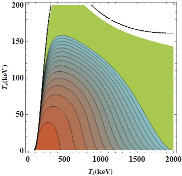
I plotted sol[[2]] because sol[[1]] corresponds to negative contour levels.
EDIT
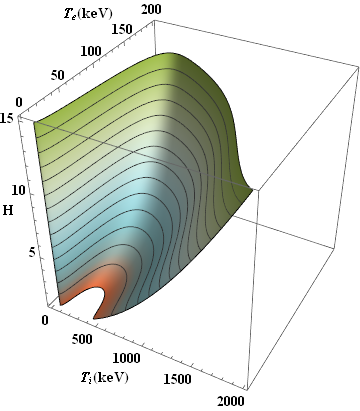
It is possible also plot this eq in 3D:
ContourPlot3D[eq == 0, {Ti, 1, 2000}, {Te, 1, 200}, {H, 1, 15}, MeshFunctions -> (#3 &), Mesh -> {Range[15]}, AxesLabel -> {Style["\!\(\*SubscriptBox[\(T\), \(i\)]\)(keV)", FontSize -> 14, FontFamily -> "Times"], Style["\!\(\*SubscriptBox[\(T\), \(e\)]\)(keV)", FontSize -> 14, FontFamily -> "Times"], Style["H", FontSize -> 14, FontFamily -> "Times"]}, LabelStyle -> Directive[Black, Bold], BaseStyle -> Directive[Black, Bold, FontSize -> 14, FontFamily -> "Times"], ColorFunction -> (ColorData["IslandColors"][#3] &)]
EDIT 2
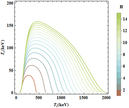
Without solving original equation eq for H, we can plot contours of eq == 0 for specific values of H:
ClearAll[eq]; eq[H_] := -1.94178*10^24*H*Te^0.5 - (3.2*(7.33376*10^27*Te^(7/2) + 4.66533*10^24*Ti^(7/2)))/ (10^9*H) + 7.68161*10^40*H*(5.41/((10^15*E^(148/Ti))*Ti^(3/2)) + 2.00122/((10^10*E^((53.124*(1 - (-0.059357*Ti + 0.0010404*Ti^2 - (9.1653*Ti^3)/10^6)/ (1 + 0.20165*Ti + 0.0027621*Ti^2 + (9.8305*Ti^3)/10^7))^(1/3))/Ti^(1/3)))* (Ti^(2/3)*(1 - (-0.059357*Ti + 0.0010404*Ti^2 - (9.1653*Ti^3)/10^6)/ (1 + 0.20165*Ti + 0.0027621*Ti^2 + (9.8305*Ti^3)/10^7))^(5/6)))); ContourPlot[Evaluate@eq[Range[15]], {Ti, 1, 2000}, {Te, 1, 200}, ContourStyle -> ColorData["IslandColors"] /@ Rescale[Range[15]], PlotLegends -> BarLegend[{"IslandColors", {1, 15}}, Range[15], LegendLabel -> "H", LegendMarkerSize -> 300, LabelStyle -> Directive[Black, Bold, FontFamily -> "Times", 14]], FrameStyle -> Directive[Black, Bold, 14, FontFamily -> "Times"], FrameLabel -> {"\!\(\*SubscriptBox[\(T\), \(i\)]\)(keV)", "\!\(\*SubscriptBox[\(T\), \(e\)]\)(keV)"}, PlotPoints -> 50]
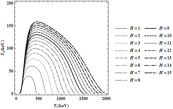
For b&w plot one can use ContourStyle option and adjust thickness and dashing (here I borrowed dashing patterns from PlotTheme -> "Monochrome" and added two types of thickness):
ContourPlot[Evaluate@eq[Range[15]], {Ti, 1, 2000}, {Te, 1, 200}, ContourStyle -> Directive @@@ Tuples[{{Black}, {Thickness[Medium], Thickness[Large]}, {AbsoluteDashing[{}], AbsoluteDashing[{6, 2}], AbsoluteDashing[{2, 2}], AbsoluteDashing[{6, 2, 2, 2}], AbsoluteDashing[{12, 2}], AbsoluteDashing[{12, 2, 2, 2, 2, 2}], AbsoluteDashing[{24, 2, 8, 2}], AbsoluteDashing[{24, 2, 2, 2}]}}], PlotLegends -> (Row[{HoldForm@H, "\[ThinSpace]=\[ThinSpace]", #}] & /@ Range[15]), FrameStyle -> Directive[Black, Bold, 14, FontFamily -> "Times"], FrameLabel -> {"\!\(\*SubscriptBox[\(T\), \(i\)]\)(keV)", "\!\(\*SubscriptBox[\(T\), \(e\)]\)(keV)"}, PlotPoints -> 50, LabelStyle -> Directive[Black, Bold, FontFamily -> "Times", 14]]