I might as well elaborate on my comment. Here is a modification of Stan Wagon's FindAllCrossings[] function (from his book Mathematica in Action, second edition) that uses Plot[] to generate the initial approximations to be subsequently polished by FindRoot[]:
Options[FindAllCrossings] = Sort[Join[Options[FindRoot], {MaxRecursion -> Automatic, PerformanceGoal :> $PerformanceGoal, PlotPoints -> Automatic}]]; FindAllCrossings[f_, {t_, a_, b_}, opts___] := Module[{r, s, s1, ya}, {r, ya} = Transpose[First[Cases[Normal[ Plot[f, {t, a, b}, Method -> Automatic, Evaluate[Sequence @@ FilterRules[Join[{opts}, Options[FindAllCrossings]], Options[Plot]]]]], Line[l_] :> l, Infinity]]]; s1 = Sign[ya]; If[ ! MemberQ[Abs[s1], 1], Return[{}]]; s = Times @@@ Partition[s1, 2, 1]; If[MemberQ[s, -1] || MemberQ[Take[s, {2, -2}], 0], Union[Join[Pick[r, s1, 0], Select[t /. Map[FindRoot[f, {t, r[[#]], r[[# + 1]]}, Evaluate[Sequence @@ FilterRules[Join[{opts}, Options[FindAllCrossings]], Options[FindRoot]]]] &, Flatten[Position[s, -1]]], a <= # <= b &]]], {}]]
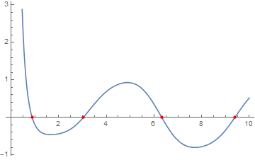
Try it out:
FindAllCrossings[BesselJ[1, x]^2 + BesselK[1, x]^2 - Sin[Sin[x]], {x, 0, 100}, WorkingPrecision -> 20] {0.88660463531346207679, 3.0329660890136683539, 6.3239665137114782212, 9.3911434075850854017, 12.589067252797192964, 15.687789316501627036, 18.865248000326751595, 21.976728589463954937, 25.144727536576135544, 28.263111694495812775, 31.425621611972587076, 34.548333253230934213, 37.707250582575859710, 40.832929091244028281, 43.989309899299199529, 47.117149292753968158, 50.271642808648651326, 53.401126310508732375, 56.554160423425108364, 59.684936863656120488, 62.836808589969946989, 65.968628466404205710, 69.119552435670107405, 72.252232119042699356, 75.402368490602128759, 78.535768909563822046, 81.685240379776511855, 84.819253682565487033, 87.968156330842562535, 91.102697190752433240, 94.251107663305908556, 97.386107414041584404}
A different implementation involves the use of the MeshFunctions option of Plot[] to generate the seeds. Here's how it looks:
FindAllCrossings[f_, {t_, a_, b_}, opts : OptionsPattern[]] := Module[{r}, r = Cases[Normal[Plot[f, {t, a, b}, MeshFunctions -> (#2 &), Mesh -> {{0}}, Method -> Automatic, Evaluate[Sequence @@ FilterRules[Join[{opts}, Options[FindAllCrossings]], Options[Plot]]]]], Point[p_] :> SetPrecision[p[[1]], OptionValue[WorkingPrecision]], Infinity]; If[r =!= {}, Union[Select[t /. Map[FindRoot[f, {t, #}, Evaluate[Sequence @@ FilterRules[Join[{opts}, Options[FindAllCrossings]], Options[FindRoot]]]] &, r], a <= # <= b &]], {}]]
This version might be a bit faster in some cases, but it no longer has the safety feature of root bracketing in the previous version.


Plot[]to find initial approximations forFindRoot[]. If you're interested in that approach, I can write up an answer. $\endgroup$Reduce[]-based methods: all of these hinge on the fact thatReduce[]apparently knows quite a fair bit about the transcendental functions built within Mathematica. If, however, you are dealing with a black-box function that can only evaluate at numerical values (you can simulate this behavior with something likef[x_?NumericQ] := Haversine[Pi x]), thenReduce[]won't be able to do much. $\endgroup$