Definition
GaussCurvature[f_] := With[{dfu = D[f, u], dfv = D[f, v]}, Simplify[(Det[{D[dfu, u], dfu, dfv}] Det[{D[dfv, v], dfu, dfv}] - Det[{D[f, u, v], dfu, dfv}]^2) / (dfu.dfu dfv.dfv - (dfu.dfv)^2)^2]];
Sphere
As @ ubpdqn already remarked
GaussCurvature[{Cos[u] Sin[v], Sin[u] Sin[v], Cos[v]}]
1
Ellipsoid
ellipsoid = {2 Cos[u] Sin[v], Sin[u] Sin[v], Cos[v]}; cur = GaussCurvature[ellipsoid]

plo = Plot3D[cur, {u, 0, Pi}, {v, 0, 2 Pi}, ColorFunction -> "TemperatureMap", PlotRange -> Full]

range = Last[PlotRange /. AbsoluteOptions[plo, PlotRange]]
{0.25, 4.}
ParametricPlot3D[ellipsoid, {u, 0, Pi}, {v, 0, 2 Pi}, Mesh -> False, ColorFunction -> Function[{x, y, z, u, v}, ColorData["TemperatureMap"][Rescale[cur, range]]], ColorFunctionScaling -> False]

Torus
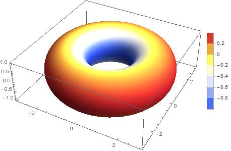
torus = {(2 + Cos[v]) Cos[u], (2 + Cos[v]) Sin[u], Sin[v]}; cur = GaussCurvature[torus]

plo = Plot3D[cur, {u, 0, 2 Pi}, {v, 0, 2 Pi}, ColorFunction -> "TemperatureMap", PlotRange -> Full]
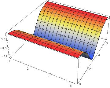
range = Last[PlotRange /. AbsoluteOptions[plo, PlotRange]]
{-1., 0.333333}
par = ParametricPlot3D[ torus, {u, 0, 2 Pi}, {v, 0, 2 Pi}, ImageSize -> 400, Mesh -> False, ColorFunction -> Function[{x, y, z, u, v}, ColorData["TemperatureMap"][Rescale[cur, range]]], ColorFunctionScaling -> False, PlotPoints -> 70]; bar = BarLegend[{"TemperatureMap", range}, Automatic]; Row[{par, bar}]
Moebius with gaussian mesh lines
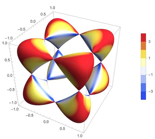
f = {Cos[v] (3 + u Cos[v/2]), Sin[v] (3 + u Cos[v/2]), u Sin[v/2]}; cur = GaussCurvature[f]; ParametricPlot3D[f, {u, -1.5, 1.5}, {v, 0, 2 Pi}, Boxed -> False, PlotStyle -> Opacity[0.8], ImageSize -> 500, Mesh -> 12, PlotPoints -> 120, MeshFunctions -> Function[{x, y, z, u, v}, Rescale[cur, {-0.04, -0.02}]], ColorFunction -> Function[{x, y, z, u, v}, ColorData["DarkRainbow"][Rescale[cur, {-0.04, -0.02}]]], ColorFunctionScaling -> False]

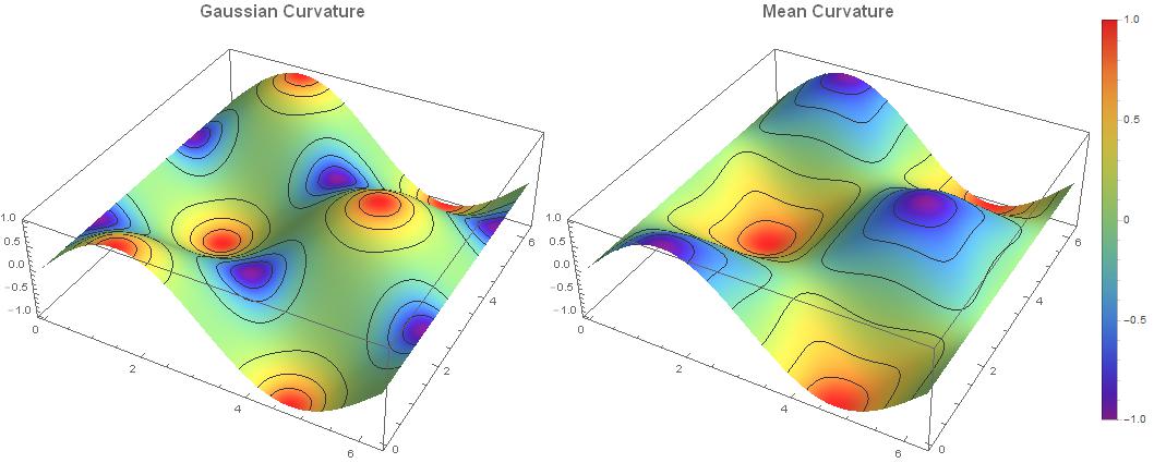
Comparison with Mean Curvature
A must-read about those jolly times: http://en.wikipedia.org/wiki/Sophie_Germain
sincos = {u, v, Sin[u] Cos[v]}; cur = GaussCurvature[sincos]; range = Last[PlotRange /. AbsoluteOptions[plo, PlotRange]]; p1 = ParametricPlot3D[sincos, {u, 0, 2 Pi}, {v, 0, 2 Pi}, ImageSize -> 500, Mesh -> 6, PlotLabel -> Style["Gaussian Curvature\n", 16, Bold], PlotPoints -> 120, MeshFunctions -> Function[{x, y, z, u, v}, Rescale[cur, range]], ColorFunction -> Function[{x, y, z, u, v}, ColorData["Rainbow"][Rescale[cur, range]]], ColorFunctionScaling -> False]; MeanCurvature[f_] := With[{du = D[f, u], dv = D[f, v]}, Simplify[(Det[{D[du, u], du, dv}] * dv.dv - 2 Det[{D[f, u, v], du, dv}] * du.dv + Det[{D[dv, v], du, dv}] * du.du) / (2 Simplify[(du.du*dv.dv - (du.dv)^2)]^(3/2))]]; cur = MeanCurvature[sincos]; plo = Plot3D[cur, {u, 0, 2 Pi}, {v, 0, 2 Pi}]; range = Last[PlotRange /. AbsoluteOptions[plo, PlotRange]]; p2 = ParametricPlot3D[sincos, {u, 0, 2 Pi}, {v, 0, 2 Pi}, ImageSize -> 500, Mesh -> 6, PlotLabel -> Style["Mean Curvature\n", 16, Bold], PlotPoints -> 120, MeshFunctions -> Function[{x, y, z, u, v}, Rescale[cur, range]], ColorFunction -> Function[{x, y, z, u, v}, ColorData["Rainbow"][Rescale[cur, range]]], ColorFunctionScaling -> False]; Row[{p1, p2, BarLegend[{"Rainbow", range}, LegendMarkerSize -> 400]}]
Update for space curves
curvature[f_] := With[{d1 = D[f, u], d2 = D[f, {u, 2}]}, Norm[Cross[d1, d2]] / Norm[d1]^3 // Simplify] loxodromes[a_, b_] := { 2 a E^(b u) Cos[u], 2 a E^(b u) Sin[u], a^2 E^(2 b u) - 1 } / (1 + a^2 E^(2 b u)) cur = curvature[loxodromes[1, 0.1]]; plo = Plot[cur, {u, -4 Pi, 4 Pi}, PlotRange -> All]

range = Last[PlotRange /. AbsoluteOptions[plo, PlotRange]]; Show[ ParametricPlot3D[loxodromes[1, 0.1], {u, -4 Pi, 4 Pi}, ColorFunction -> Function[{x, y, z, u, v}, ColorData["Rainbow"][Rescale[cur, range]]], ColorFunctionScaling -> False, PlotStyle -> Thickness[0.01]], Graphics3D[{Opacity[0.2], Sphere[]}], ImageSize -> 500]

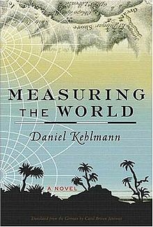
A nice novel about Gauss


FrenetSerretSystemandArcCurvaturebut they compute curvature of curves only. See e.g. this Finding unit tangent.... In general on a manifold (e.g. surface) you can compute Gauss curvature calculating Christoffel Symbols see e.g. How to calculate Ricci curvature and Christoffel $\endgroup$