I have been attempting to port a modified version of the Yakopcic memristor from Python/MATLAB to LTspice but have been running into issues with the results not being the same, as shown in the following pictures.
In Python/MATLAB the memristor is simulated by using Euler's method to solve the IVP describing the device's internal state evolution.
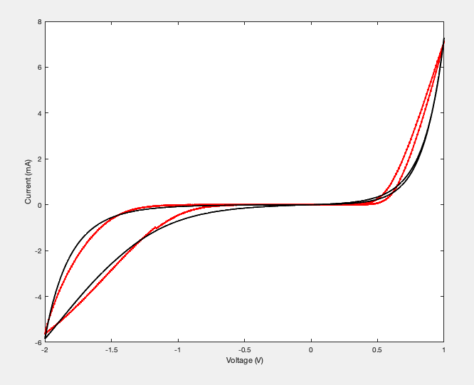
MATLAB simulation result
[ ]
]
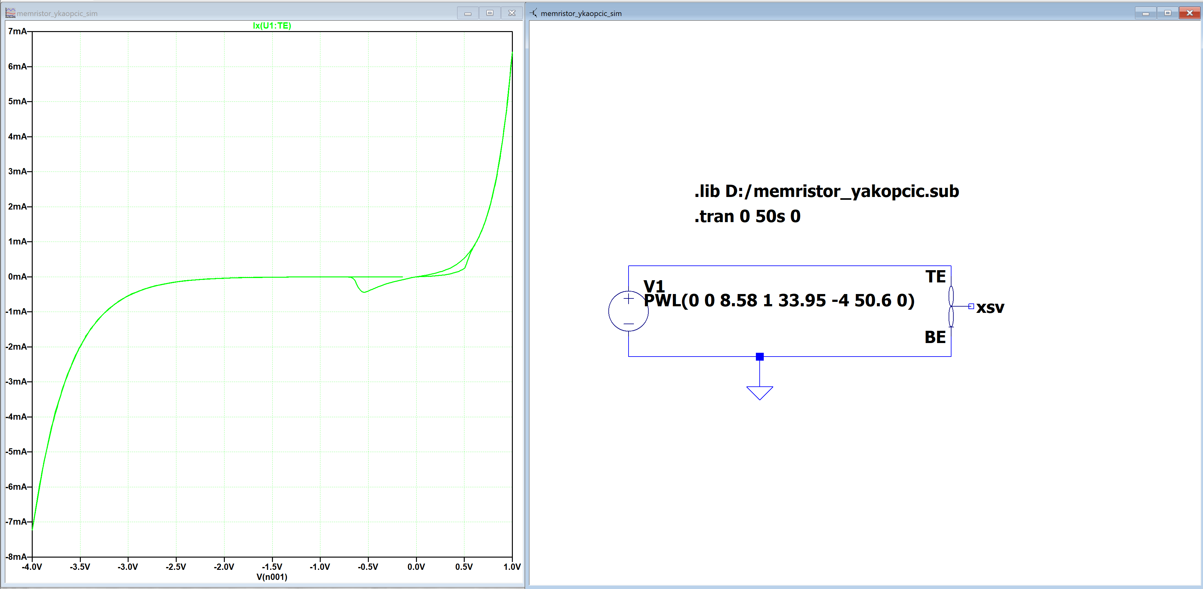
LTspice simulation result
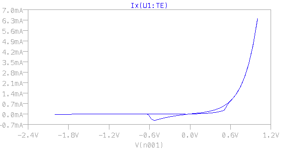
I think that this answer may have put me on the right track (https://electronics.stackexchange.com/a/368910/294242) by pointing out that timing in the SPICE engine could lead to issues.
In fact, if I enlarge my timestep from dt=1/10000 to dt=1 in MATLAB/Python, I get the same exact result as in LTspice.
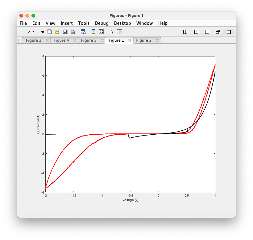
MATLAB simulation with dt=1 (the curve in black)
Is there any way to solve the issue I'm seeing? I have tried .tran 0 50s 0 {1/10000} to match dt=1/10000, but the results don't change.
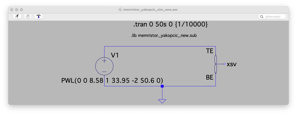
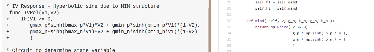
* SPICE model for memristive devices * Created by Chris Yakopcic * Last Update: 8/9/2011 * * Connections: * TE - top electrode * BE - bottom electrode * XSV - External connection to plot state variable * that is not used otherwise .subckt MEM_YAKOPCIC TE BE XSV * Fitting parameters to model different devices * gmax_p, bmax_p, gmax_n, bmax_n: Parameters for OFF state IV relationship * gmin_p, bmin_p, gmin_n, bmin_n: Parameters for OFF state IV relationship * Vp, Vn: Pos. and neg. voltage thresholds * Ap, An: Multiplier for SV motion intensity * xp, xn: Points where SV motion is reduced * alphap, alphan: Rate at which SV motion decays * xo: Initial value of SV * eta: SV direction relative to voltage .param gmax_p=9e-5 bmax_p=4.96 gmax_n=1.7e-4 bmax_n=3.23 + gmin_p=1.5e-5 bmin_p=6.91 gmin_n=4.4e-7 bmin_n=2.6 + Ap=90 An=10 + Vp=0.5 Vn=0.5 + xp=0.1 xn=0.242 + alphap=1 alphan=1 + xo=0 eta=1 * Multiplicative functions to ensure zero state * variable motion at memristor boundaries .func wp(V) = xp/(1-xp) - V/(1-xp) + 1 .func wn(V) = V/xn * Function G(V(t)) - Describes the device threshold .func G(V) = + IF(V > Vp, + Ap*(exp(V)-exp(Vp)), + IF(V < -Vn, + -An*(exp(-V)-exp(Vn)), + 0 ) ) * Function F(V(t),x(t)) - Describes the SV motion .func F(V1,V2) = + IF(eta*V1 >= 0, + IF(V2 >= xp, + exp(-alphap*(V2-xp))*wp(V2), + 1 ), + IF(V2 <= xn, + exp(alphan*(V2-xn))*wn(V2), + 1 ) ) * IV Response - Hyperbolic sine due to MIM structure .func IVRel(V1,V2) = + IF(V1 >= 0, + gmax_p*sinh(bmax_p*V1)*V2 + gmin_p*sinh(bmin_p*V1)*(1-V2), + gmax_n*sinh(bmax_n*V1)*V2 + gmin_n*sinh(bmin_n*V1)*(1-V2) + ) * Circuit to determine state variable * dx/dt = F(V(t),x(t))*G(V(t)) Cx XSV 0 {1} .ic V(XSV) = xo Gx 0 XSV value={eta*F(V(TE,BE),V(XSV,0))*G(V(TE,BE))} * Current source for memristor IV response Gm TE BE value = {IVRel(V(TE,BE),V(XSV,0))} .ends MEM_YAKOPCIC EDIT: It turns out that the issue was not in the MATLAB to SPICE porting but rather in the original MATALB script itself. The MATLAB/Python script did not use a the same timestep as the real simulation.
I measured the experimental timestep and found it to be dt~=0.08s, so by using Euler with dt=1/10000 the MATLAB script was effectively simulating for only 60 ms, instead of the 50 s in the real experiment. Scaling the Ap and An parameters to match the updated - much larger - timestep was enough to reproduce the experimental results.
trapezoidal,modified trapezoidal, andGearintegration with no discernible outcomes. I also tried switching the solver fromNormaltoAlternate, again to no avail. I've also tried alternate solvers in Python (for ex.,LSODA,RK4) and the results are the same as plain FE. (also, Yakopcic uses FE in his MATLAB simulations) \$\endgroup\$