So I'm trying to fit experimental data to a nonlinear model using the NonLinearModelFit command, but it isn't quite working.
The plotted data set looks like this:
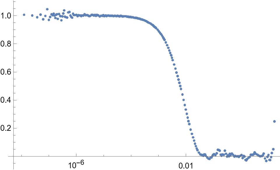
The data is to be fitted with
1+β*exp(-2γ*t), so I tried using the NonLinearModelFit command as follows:
nlm = NonlinearModelFit[data, 1 + beta*Exp[-2 gamma*t], {beta, gamma}, t]; LogLinearPlot[nlm[t], {t, 0, data[[Length[data], 1]]}, PlotRange -> Automatic] Show[ListLogLinearPlot[data], LogLinearPlot[nlm[t], {t, 0, data[[Length[data], 1]]}, PlotStyle -> Red]] which looks like

The proposed function obviously doesn't fit the data set and is a scaled down version shifted to the right, without the last almost constant part of the data.
What's happening here? How can I accurately fit the data and maybe use some initial values for the parameters β and γ?
The data used to plot and fit:
082222 1251 PM Experiment Type Sizing Pseudo Cross Correlation Scattering angle 40.0 Duration (s) 20 Wavelength (nm) 660.0 Refractive index 1.330 Viscosity (mPas) 1.000 Temperature (K) 293.2 Laser intensity (mW) 0.147463 Average Count rate A (kHz) 191.3 Average Count rate B (kHz) 192.1 Intercept 0.9941 Cumulant 1st 667.97 Cumulant 2nd 667.97 0.00 Cumulant 3rd 641.63 0.40 Lag time (s) g2-1 1.250000E-8 0.981694 2.500000E-8 0.991310 3.750000E-8 0.987267 5.000000E-8 0.986830 6.250000E-8 0.995900 7.500000E-8 0.988141 8.750000E-8 0.985300 1.000000E-7 1.028684 1.125000E-7 0.977760 1.250000E-7 1.000162 1.375000E-7 0.988360 1.500000E-7 0.991529 1.625000E-7 0.992731 1.750000E-7 1.001255 1.875000E-7 1.003659 2.000000E-7 0.992731 2.125000E-7 0.996173 2.375000E-7 1.001583 2.625000E-7 0.976339 2.875000E-7 0.992731 3.125000E-7 1.007101 3.375000E-7 0.977377 3.625000E-7 0.994370 3.875000E-7 1.004151 4.125000E-7 0.997539 4.625000E-7 0.989972 5.125000E-7 1.003577 5.625000E-7 1.000408 6.125000E-7 0.990054 6.625000E-7 0.985109 7.125000E-7 0.992977 7.625000E-7 0.994452 8.125000E-7 0.987171 9.125000E-7 1.003509 1.012500E-6 1.004055 1.112500E-6 0.994712 1.212500E-6 0.990600 1.312500E-6 0.985559 1.412500E-6 0.988237 1.512500E-6 1.000039 1.612500E-6 1.001002 1.812500E-6 0.983599 2.012500E-6 0.993154 2.212500E-6 0.994131 2.412500E-6 0.994090 2.612500E-6 0.997109 2.812500E-6 0.998311 3.012500E-6 0.997553 3.212500E-6 0.993281 3.612500E-6 0.994408 4.012500E-6 0.989310 4.412500E-6 0.996071 4.812500E-6 0.993520 5.212500E-6 0.990286 5.612500E-6 0.992212 6.012500E-6 0.992093 6.412500E-6 0.992017 7.212500E-6 0.994756 8.012500E-6 0.994418 8.812500E-6 0.991991 9.612500E-6 0.990677 1.041250E-5 0.991290 1.121250E-5 0.995478 1.201250E-5 0.993559 1.281250E-5 0.996065 1.441250E-5 0.996347 1.601250E-5 0.991484 1.761250E-5 0.990913 1.921250E-5 0.993117 2.081250E-5 0.991552 2.241250E-5 0.990403 2.401250E-5 0.991326 2.561250E-5 0.991138 2.881250E-5 0.991134 3.201250E-5 0.991837 3.521250E-5 0.990236 3.841250E-5 0.990808 4.161250E-5 0.989931 4.481250E-5 0.990017 4.801250E-5 0.990026 5.121250E-5 0.988744 5.761250E-5 0.987654 6.401250E-5 0.987021 7.041250E-5 0.986750 7.681250E-5 0.985235 8.321250E-5 0.985939 8.961250E-5 0.985592 9.601250E-5 0.985029 0.000102 0.984424 0.000115 0.982993 0.000128 0.982606 0.000141 0.980761 0.000154 0.978720 0.000166 0.978311 0.000179 0.977051 0.000192 0.975604 0.000205 0.974399 0.000230 0.972358 0.000256 0.969710 0.000282 0.966684 0.000307 0.965229 0.000333 0.961571 0.000358 0.960360 0.000384 0.957262 0.000410 0.955180 0.000461 0.950771 0.000512 0.945581 0.000563 0.941056 0.000614 0.936345 0.000666 0.931493 0.000717 0.927869 0.000768 0.922947 0.000819 0.918401 0.000922 0.908841 0.001024 0.899845 0.001126 0.890876 0.001229 0.881773 0.001331 0.873013 0.001434 0.864277 0.001536 0.855824 0.001638 0.847578 0.001843 0.830522 0.002048 0.814198 0.002253 0.798193 0.002458 0.782513 0.002662 0.767277 0.002867 0.752026 0.003072 0.736805 0.003277 0.721951 0.003686 0.693111 0.004096 0.665850 0.004506 0.640100 0.004915 0.615177 0.005325 0.591402 0.005734 0.569494 0.006144 0.548935 0.006554 0.529993 0.007373 0.493404 0.008192 0.458930 0.009011 0.425248 0.009830 0.394020 0.010650 0.364432 0.011469 0.337440 0.012288 0.311853 0.013107 0.287955 0.014746 0.243217 0.016384 0.205101 0.018022 0.173352 0.019661 0.144798 0.021299 0.120097 0.022938 0.098263 0.024576 0.079198 0.026214 0.064734 0.029491 0.041283 0.032768 0.024546 0.036045 0.009757 0.039322 -0.007328 0.042598 -0.023800 0.045875 -0.027768 0.049152 -0.025468 0.052429 -0.020721 0.058982 0.002437 0.065536 0.022033 0.072090 0.038237 0.078643 0.044000 0.085197 0.025870 0.091750 0.002250 0.098304 -0.003367 0.104858 -0.018009 0.117965 -0.031016 0.131072 -0.029388 0.144179 -0.026414 0.157286 -0.028317 0.170394 -0.016462 0.183501 0.007269 0.196608 0.010597 0.209715 0.015417 0.235930 0.019428 0.262144 0.020318 0.288358 0.032608 0.314573 0.035763 0.340787 0.022082 0.367002 -0.006260 0.393216 0.004914 0.419430 0.007707 0.471859 -0.005449 0.524288 0.006633 0.576717 -0.004173 0.629146 0.007739 0.681574 -0.001696 0.734003 0.000670 0.786432 0.001787 0.838861 -0.009630 0.943718 -0.003229 1.048576 -0.003674 1.153434 -0.011465 1.258291 0.010513 1.363149 -0.031880 1.468006 -0.017126 1.572864 0.004514 1.677722 -0.003074 1.887437 0.000161 2.097152 -0.005843 2.306867 -0.007362 2.516582 0.012358 2.726298 0.011785 2.936013 0.028037 3.145728 0.024937 3.355443 0.019830 3.774873 0.004959 4.194304 0.009447 4.613734 0.028008 5.033165 0.031347 5.452595 0.021929 5.872025 0.046492 6.291456 0.031570 6.710886 0.027511 7.549747 0.018476 8.388608 0.043572 9.227468 0.068573 10.066330 0.027640 10.905190 0.042270 11.744051 0.065827 12.582912 0.064546 13.421773 0.053715 15.099494 0.105235 16.777216 -0.051853 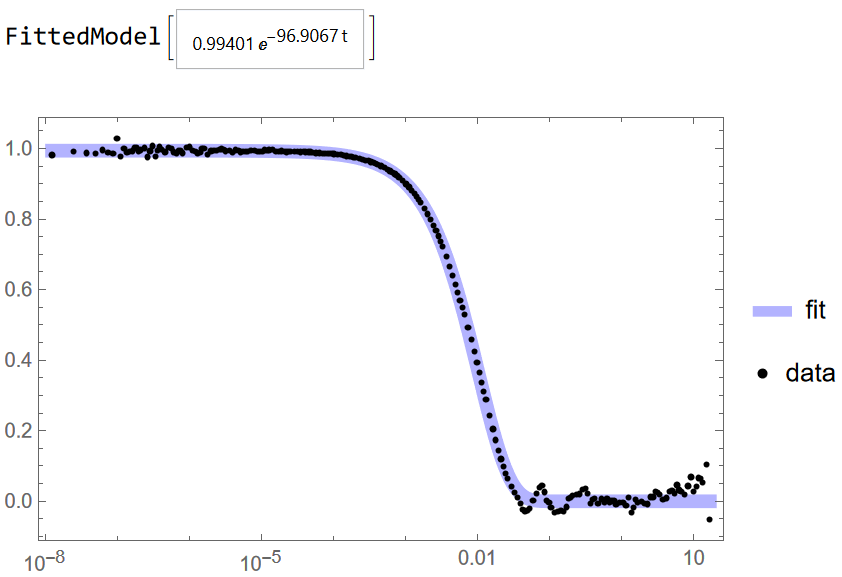
1+β*exp(-2γ*t), say the tails. $\endgroup$t<10^-6, but it just shifted the fitted function a tiny bit in negative y direction $\endgroup$