Introduction
I worked up my solution and then saw that Jens had suggested this approach in a comment. Well, here's my approach. It is fairly general. I made no attempt to determine how many connected components there are and finding parametrizations of each one.
Find a point on the intersection. This could be a difficult step, depending on how much is known about the surfaces.
- A known point.
- Use
Solve or NSolve, if they work. One might be able to solve one variable in terms of the others or use a hyperplane that intersects the intersection of the surfaces. - Use root-finding, provided a feasible starting point is known. I'll give a pseudo-Newton's Method function for hunting down an intersection point below.
Integrate the normalized cross product of the gradients of the function {f, g} that define the surfaces {f == 0, g == 0}. Since the cross product is perpendicular to both gradients of f and g, it will be tangent to the intersection curve. Using the normalized vector yields a unit-speed parametrization. This is fairly easy with NDSolve.
- Determining the limits of integration usually needs some user-input.
- We can get a periodic interpolation of closed curves.
Utility functions
findPoint[{f, g}, {{x, y, z}, {x0, y0, z0}}] - finds a point on the intersection of {f == 0, g == 0}, starting at {x0, y0, z0}. It uses Newton-Method-like step pseudonewton.
periodicEvent[v, v0, p0] - stops integration when the solution has completed a loop, using the condition v == v0 to trigger the event; p0 should be the initial point and v0 should be the corresponding coordinate.
findIntersection3D[{f, g}, {{x, y, z}, {x0, y0, z0}}, {t, t1, t2}] - finds a parametrization of the intersection of {F == 0, g == 0} near the point {x0, y0, z0}.
periodicReinterpolation[if] - converts the InterpolatingFunction if to a periodic one. Just something "extra"; it plays no crucial role.
showall[{f, g}, sol] - another "extra," which shows the plots of f == 0, g == 0, and the intersection parametrized by sol.
Examples
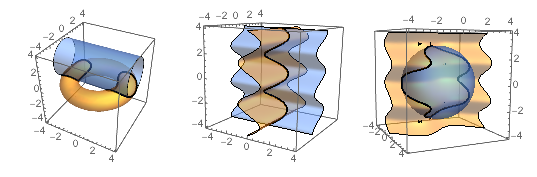
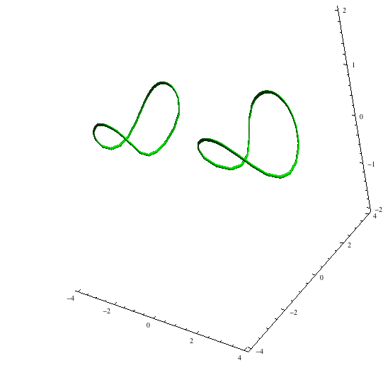
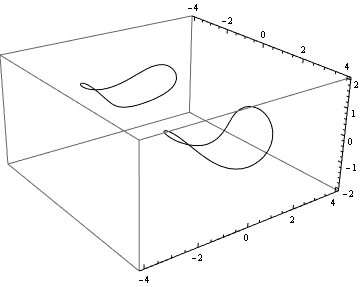
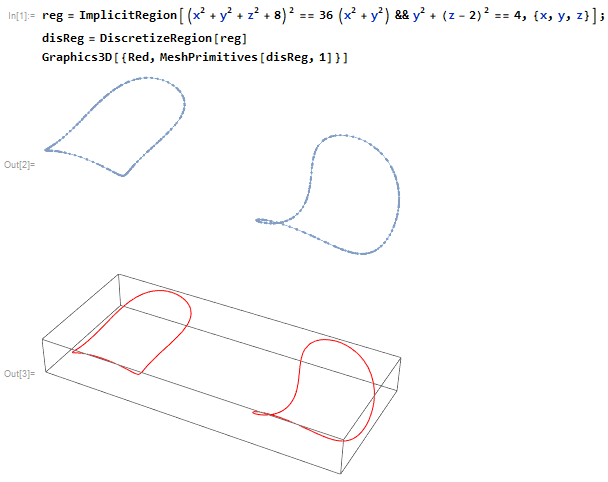
The three examples below were each shown with showall[{f, g}, sol].
OP's example. Converting to a periodic interpolation is not necessary; it is done merely to show it can be done.
{f, g} = {(x^2 + y^2 + z^2 + 8)^2 - 36 (x^2 + y^2), y^2 + (z - 2)^2 - 4}; sol = findIntersection3D[{f, g}, {{x, y, z}, #}, {t, 0, 100}, "EventFunctions" -> {periodicEvent[y[t], #[[2]], #] &}] & /@ {{-4, 0, 0}, {4, 0, 0}} /. if_InterpolatingFunction :> periodicReinterpolation[if];
Helix. OK, paramterization by hand is easy, but I've always liked this construction of the helix as the intersection of two corrugated sheets. I used Solve to find the point of intersection at the bottom of the plot range (z == -4). It's actually shorter to write it out explicitly, but in principle
{f, g} = {x - Cos[2 z], y - Sin[2 z]}; sol = findIntersection3D[{f, g}, {{x, y, z}, {x, y, z} /. First@Solve[{z == -4, {x - Cos[2 z], y - Sin[2 z]} == {0, 0}}}, {t, 0, 100}, "EventFunctions" -> {WhenEvent[z[t] == 4, "StopIntegration"] &}];
A somewhat random transcendental surface and sphere.
{f, g} = {x + Sin[y] + Cos[2 z], x^2 + y^2 + z^2 - 9}; sol = findIntersection3D[{f, g}, {{x, y, z}, {0, 0, 2}}, {t, 0, 100}, "EventFunctions" -> {periodicEvent[x[t], First[#], #] &}];
Code
Root-finding. I have not seen Newton's Method used on an underdetermined system, but that's basically that findPoint does. In the main function, findPoint starts the search at the point {x0, y0, z0} passed to findIntersection3D.
ClearAll[findPoint, pseudonewton, periodicEvent, findIntersection3D, periodicReinterpolation, showall]; pseudonewton[f_List, {x_, y_, z_}] := pseudonewton[f, D[f, {{x, y, z}}], {x, y, z}]; pseudonewton[f_List, df_?MatrixQ, {x_, y_, z_}] := With[{df0 = df /. Thread[{x, y, z} -> #], f0 = f /. Thread[{x, y, z} -> #]}, # - PseudoInverse[df0].f0] &; findPoint[f_List, {{x_, y_, z_}, {x0_, y0_, z0_}}] := NestWhile[pseudonewton[f, D[f, {{x, y, z}}], {x, y, z}], {x0, y0, z0}, Norm[f /. Thread[{x, y, z} -> #]] > 1*^-15 &, 2, 100];
Constructing the intersection. Although one specifies an interval {t, t1, t2} in calling findIntersection3D (see above, Utility functions), events are probably the easiest way to control the interval of integration. The option "EventFunctions" -> list takes a list of functions whose input is the starting point found by findPoint. They should output an WhenEvent expression. The function periodicEvent returns a event function that detects when the path computed by NDSolve returns to its starting position. When the variable v equals the number v0 and the point {x[t], y[t], z[t]}, is close to the starting point p0, integration stops; the number v0 should be the corresponding coordinate of p0. In certain cases, periodicEvent might need tweaking. The condition that the distance be within 0.1 is coordinated with the option MaxStepSize -> 0.1 in NDSolve. If the step size is greater, the event may be missed. It can also happen that the starting point p0 is at an extreme value of the variable v that periodicEvent tracks. Either change the variable or pass a periodicEvent for two or three variables.
periodicEvent[v_, v0_, p0_] := WhenEvent[v == v0 && Norm[{x[t], y[t], z[t]} - p0] < 0.1, "StopIntegration"]; Options[findIntersection3D] = Join[{"EventFunctions" -> {}}, Options[NDSolve]]; findIntersection3D[funcs : {_, _}, {{x_, y_, z_}, {x0_, y0_, z0_}}, {t_, t1_, t2_}, opts : OptionsPattern[]] := Module[{vel, eqn, ics, invariants}, vel = Cross @@ D[funcs, {{x, y, z}}] // Normalize; eqn = {x'[t], y'[t], z'[t]} == (vel /. {v : x | y | z :> v[t]}); ics = findPoint[funcs, {{x, y, z}, N@{x0, y0, z0}}]; invariants = funcs /. {v : x | y | z :> v[t]}; First@NDSolve[{ eqn, {x[0], y[0], z[0]} == ics, Through[OptionValue["EventFunctions"][ics]]}, {x, y, z}, {t, 0, 100}, FilterRules[{opts}, Options[NDSolve]], MaxStepSize -> 0.1, Method -> {"Projection", "Invariants" -> invariants}] ];
Extras.
showall[{f_, g_}, sol_] := Show[ ContourPlot3D[{f == 0, g == 0}, {x, -4, 4}, {y, -4, 4}, {z, -4, 4}, ContourStyle -> Opacity[0.5], Mesh -> None], ParametricPlot3D[{x[t], y[t], z[t]} /. sol // Evaluate, Evaluate@Join[{t}, Flatten[x["Domain"] /. First@sol]], PlotStyle -> Black] ]; periodicReinterpolation[if_InterpolatingFunction] := Module[{coords = First@if["Coordinates"], values = if["ValuesOnGrid"]}, If[Chop@First@Differences[if /@ Flatten[if["Domain"]]] != 0, Print["Warning: The endpoints are significantly different."]]; values[[-1]] = values[[1]]; Interpolation[Transpose@{coords, values}] ];
BSplinesurfaces that has no explicit analytical form? This will be very effective for 3D modeling. $\endgroup$BSplineSurface[]objects can be transformed intoBSplineFunction[]s). $\endgroup$t[r], where r is a 3D point). Then the curve is described byD[r[u],u] == t[r[u]]for curve parameteru. This is becausetmust be tangent to both surfaces for all pointsron the intersection curve. You "just" have to integrate that equation with a starting pointr0on the intersection. $\endgroup$