replaced http://mathematica.stackexchange.com/ with https://mathematica.stackexchange.com/
Source Link

Borrowing almost verbatim from a recent response about finding extremaextrema, here is a method that is useful when your function is differentiable and hence can be "tracked" by NDSolve.

f[x_] := BesselJ[1, x]^2 + BesselK[1, x]^2 - Sin[Sin[x]] In[191]:= zeros = Reap[soln = y[x] /. First[ NDSolve[{y'[x] == Evaluate[D[f[x], x]], y[10] == (f[10])}, y[x], {x, 10, 0}, Method -> {"EventLocator", "Event" -> y[x], "EventAction" :> Sow[{x, y[x]}]}]]][[2, 1]] During evaluation of In[191]:= NDSolve::mxst: Maximum number of 10000 steps reached at the point x == 1.5232626281716416`*^-124. >> Out[191]= {{9.39114, 8.98587*10^-16}, {6.32397, -3.53884*10^-16}, {3.03297, -8.45169*10^-13}, {0.886605, -4.02456*10^-15}} Plot[f[x], {x, 0, 10}, Epilog -> {PointSize[Medium], Red, Point[zeros]}] 

function and roots

If it were a trickier function, one might use Method -> {"Projection", ...} to enforce the condition that y[x] is really the same as f[x]. This method may be useful in situations (if you can find them) where we have one function in one variable, and Reduce either cannot handle it or takes a long time to do so.


Addendum by J. M.

WhenEvent is now the documented way to include event detection in NDSolve, so using it along with the trick of specifying an empty list where the function should be, here's how to get a pile of zeroes:

f[x_] := BesselJ[1, x]^2 + BesselK[1, x]^2 - Sin[Sin[x]] zeros = Reap[NDSolve[{y'[x] == D[f[x], x], WhenEvent[y[x] == 0, Sow[{x, y[x]}]], y[10] == f[10]}, {}, {x, 10, 0}]][[-1, 1]]; Plot[f[x], {x, 0, 10}, Epilog -> {PointSize[Medium], Red, Point[zeros]}] 
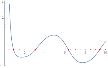
function and roots

Borrowing almost verbatim from a recent response about finding extrema, here is a method that is useful when your function is differentiable and hence can be "tracked" by NDSolve.

f[x_] := BesselJ[1, x]^2 + BesselK[1, x]^2 - Sin[Sin[x]] In[191]:= zeros = Reap[soln = y[x] /. First[ NDSolve[{y'[x] == Evaluate[D[f[x], x]], y[10] == (f[10])}, y[x], {x, 10, 0}, Method -> {"EventLocator", "Event" -> y[x], "EventAction" :> Sow[{x, y[x]}]}]]][[2, 1]] During evaluation of In[191]:= NDSolve::mxst: Maximum number of 10000 steps reached at the point x == 1.5232626281716416`*^-124. >> Out[191]= {{9.39114, 8.98587*10^-16}, {6.32397, -3.53884*10^-16}, {3.03297, -8.45169*10^-13}, {0.886605, -4.02456*10^-15}} Plot[f[x], {x, 0, 10}, Epilog -> {PointSize[Medium], Red, Point[zeros]}] 

function and roots

If it were a trickier function, one might use Method -> {"Projection", ...} to enforce the condition that y[x] is really the same as f[x]. This method may be useful in situations (if you can find them) where we have one function in one variable, and Reduce either cannot handle it or takes a long time to do so.


Addendum by J. M.

WhenEvent is now the documented way to include event detection in NDSolve, so using it along with the trick of specifying an empty list where the function should be, here's how to get a pile of zeroes:

f[x_] := BesselJ[1, x]^2 + BesselK[1, x]^2 - Sin[Sin[x]] zeros = Reap[NDSolve[{y'[x] == D[f[x], x], WhenEvent[y[x] == 0, Sow[{x, y[x]}]], y[10] == f[10]}, {}, {x, 10, 0}]][[-1, 1]]; Plot[f[x], {x, 0, 10}, Epilog -> {PointSize[Medium], Red, Point[zeros]}] 

function and roots

added 691 characters in body
Source Link

Borrowing almost verbatim from a recent response about finding extrema, here is a method that is useful when your function is differentiable and hence can be "tracked" by NDSolve.

f[x_] := BesselJ[1, x]^2 + BesselK[1, x]^2 - Sin[Sin[x]] In[191]:= zeros = Reap[soln = y[x] /. First[ NDSolve[{y'[x] == Evaluate[D[f[x], x]], y[10] == (f[10])}, y[x], {x, 10, 0}, Method -> {"EventLocator", "Event" -> y[x], "EventAction" :> Sow[{x, y[x]}]}]]][[2, 1]] During evaluation of In[191]:= NDSolve::mxst: Maximum number of 10000 steps reached at the point x == 1.5232626281716416`*^-124. >> Out[191]= {{9.39114, 8.98587*10^-16}, {6.32397, -3.53884*10^-16}, {3.03297, -8.45169*10^-13}, {0.886605, -4.02456*10^-15}} Plot[f[x], {x, 0, 10}, Epilog -> {PointSize[Medium], Red, Point[zeros]}] 

function and roots

If it were a trickier function, one might use Method -> {"Projection", ...} to enforce the condition that y[x] is really the same as f[x]. This method may be useful in situations (if you can find them) where we have one function in one variable, and Reduce either cannot handle it or takes a long time to do so.


Addendum by J. M.

WhenEvent is now the documented way to include event detection in NDSolve, so using it along with the trick of specifying an empty list where the function should be, here's how to get a pile of zeroes:

f[x_] := BesselJ[1, x]^2 + BesselK[1, x]^2 - Sin[Sin[x]] zeros = Reap[NDSolve[{y'[x] == D[f[x], x], WhenEvent[y[x] == 0, Sow[{x, y[x]}]], y[10] == f[10]}, {}, {x, 10, 0}]][[-1, 1]]; Plot[f[x], {x, 0, 10}, Epilog -> {PointSize[Medium], Red, Point[zeros]}] 

function and roots

Borrowing almost verbatim from a recent response about finding extrema, here is a method that is useful when your function is differentiable and hence can be "tracked" by NDSolve.

f[x_] := BesselJ[1, x]^2 + BesselK[1, x]^2 - Sin[Sin[x]] In[191]:= zeros = Reap[soln = y[x] /. First[ NDSolve[{y'[x] == Evaluate[D[f[x], x]], y[10] == (f[10])}, y[x], {x, 10, 0}, Method -> {"EventLocator", "Event" -> y[x], "EventAction" :> Sow[{x, y[x]}]}]]][[2, 1]] During evaluation of In[191]:= NDSolve::mxst: Maximum number of 10000 steps reached at the point x == 1.5232626281716416`*^-124. >> Out[191]= {{9.39114, 8.98587*10^-16}, {6.32397, -3.53884*10^-16}, {3.03297, -8.45169*10^-13}, {0.886605, -4.02456*10^-15}} Plot[f[x], {x, 0, 10}, Epilog -> {PointSize[Medium], Red, Point[zeros]}] 

function and roots

If it were a trickier function, one might use Method -> {"Projection", ...} to enforce the condition that y[x] is really the same as f[x]. This method may be useful in situations (if you can find them) where we have one function in one variable, and Reduce either cannot handle it or takes a long time to do so.


Addendum by J. M.

WhenEvent is now the documented way to include event detection in NDSolve, so using it along with the trick of specifying an empty list where the function should be, here's how to get a pile of zeroes:

f[x_] := BesselJ[1, x]^2 + BesselK[1, x]^2 - Sin[Sin[x]] zeros = Reap[NDSolve[{y'[x] == D[f[x], x], WhenEvent[y[x] == 0, Sow[{x, y[x]}]], y[10] == f[10]}, {}, {x, 10, 0}]][[-1, 1]]; Plot[f[x], {x, 0, 10}, Epilog -> {PointSize[Medium], Red, Point[zeros]}] 

function and roots

deleted 49 characters in body
Source Link

Borrowing almost verbatim from a recent response about finding extremaextrema, here is a method that is useful when your function is differentiable and hence can be "tracked" by NDSolveNDSolve.

f[x_] := BesselJ[1, x]^2 + BesselK[1, x]^2 - Sin[Sin[x]] In[191]:= zeros = Reap[soln = y[x] /. First[ NDSolve[{y'[x] == Evaluate[D[f[x], x]], y[10] == (f[10])}, y[x], {x, 10, 0}, Method -> {"EventLocator", "Event" -> y[x], "EventAction" :> Sow[{x, y[x]}]}]]][[2, 1]] During evaluation of In[191]:=   NDSolve::mxst: Maximum number of 10000 steps reached at the point   x == 1.5232626281716416`*^-124. >> Out[191]= {{9.39114,  8.98587*10^-16}, {6.32397, -3.53884*10^-16},  {3.03297, \ -8.45169*10^-13}, {0.886605, -4.02456*10^-15}} Plot[f[x], {x, 0, 10}, Epilog -> {PointSize[Medium], Red, Point[zeros]}] 

enter image description herefunction and roots

If it were a trickier function, one might use Method->{"Projection",...}Method -> {"Projection", ...} to enforce the condition that y[x]y[x] is really the same as f[x]f[x]. This method may be useful in situations (if you can find them) where we have one function in one variable, and ReduceReduce either cannot handle it or takes a long time to do so.

Borrowing almost verbatim from a recent response about finding extrema, here is a method that is useful when your function is differentiable and hence can be "tracked" by NDSolve.

f[x_] := BesselJ[1, x]^2 + BesselK[1, x]^2 - Sin[Sin[x]] In[191]:= zeros = Reap[soln = y[x] /. First[ NDSolve[{y'[x] == Evaluate[D[f[x], x]], y[10] == (f[10])}, y[x], {x, 10, 0}, Method -> {"EventLocator", "Event" -> y[x], "EventAction" :> Sow[{x, y[x]}]}]]][[2, 1]] During evaluation of In[191]:= NDSolve::mxst: Maximum number of 10000 steps reached at the point x == 1.5232626281716416`*^-124. >> Out[191]= {{9.39114,  8.98587*10^-16}, {6.32397, -3.53884*10^-16}, {3.03297, \ -8.45169*10^-13}, {0.886605, -4.02456*10^-15}} Plot[f[x], {x, 0, 10}, Epilog -> {PointSize[Medium], Red, Point[zeros]}] 

enter image description here

If it were a trickier function, one might use Method->{"Projection",...} to enforce the condition that y[x] is really the same as f[x]. This method may be useful in situations (if you can find them) where we have one function in one variable, and Reduce either cannot handle it or takes a long time to do so.

Borrowing almost verbatim from a recent response about finding extrema, here is a method that is useful when your function is differentiable and hence can be "tracked" by NDSolve.

f[x_] := BesselJ[1, x]^2 + BesselK[1, x]^2 - Sin[Sin[x]] In[191]:= zeros = Reap[soln = y[x] /. First[ NDSolve[{y'[x] == Evaluate[D[f[x], x]], y[10] == (f[10])}, y[x], {x, 10, 0}, Method -> {"EventLocator", "Event" -> y[x], "EventAction" :> Sow[{x, y[x]}]}]]][[2, 1]] During evaluation of In[191]:=  NDSolve::mxst: Maximum number of 10000 steps reached at the point  x == 1.5232626281716416`*^-124. >> Out[191]= {{9.39114, 8.98587*10^-16}, {6.32397, -3.53884*10^-16},  {3.03297, -8.45169*10^-13}, {0.886605, -4.02456*10^-15}} Plot[f[x], {x, 0, 10}, Epilog -> {PointSize[Medium], Red, Point[zeros]}] 

function and roots

If it were a trickier function, one might use Method -> {"Projection", ...} to enforce the condition that y[x] is really the same as f[x]. This method may be useful in situations (if you can find them) where we have one function in one variable, and Reduce either cannot handle it or takes a long time to do so.

Source Link
Daniel Lichtblau
  • 61.2k
  • 2
  • 107
  • 206
Loading