One can use Interpolation with InterpolationOrder -> 0:
SeedRandom[1]; data = RandomReal[1, 10] (* {0.817389, 0.11142, 0.789526, 0.187803, 0.241361, 0.0657388, 0.542247, 0.231155, 0.396006, 0.700474} *) nf = Evaluate@ Interpolation[Transpose@{-data, data}, InterpolationOrder -> 0, "ExtrapolationHandler" -> {With[{m = -Max[data]}, Piecewise[{{-m, # < m}}, Indeterminate] &], "WarningMessage" -> False} ][-#] &; Plot[nf[x], {x, -0.5, 1.5}, Epilog -> {Red, PointSize@Medium, Point[Transpose@{data, data}]}]
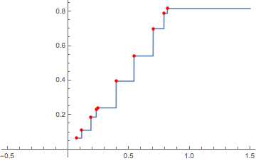
Replace Indeterminate with the value desired when the input falls below the minimum of the data.
Interpolation[] takes longer than Nearest[] to form the function, but it is faster to evaluate on large data:
SeedRandom[1]; data = RandomReal[1, 1000000]; nf = Evaluate@ Interpolation[Transpose@{-data, data}, InterpolationOrder -> 0, "ExtrapolationHandler" -> {With[{m = -Max[data]}, Piecewise[{{-m, # < m}}, Indeterminate] &], "WarningMessage" -> False} ][-#] &; // RepeatedTiming nf /@ RandomReal[1, 1000]; // RepeatedTiming (* {1.43, Null} {0.0043, Null} *) (* Sascha's distance function dist[] *) nf2 = Nearest[data, DistanceFunction -> dist]; // RepeatedTiming nf2 /@ RandomReal[1, 2]; // RepeatedTiming (* {0.000015, Null} {4.4, Null} *)
Relative speed vs. length of data to evaluate the function on an input, showing that nf becomes orders of magnitude faster as the size of data increases:
Length@data 1000 10000 100000 1000000 nf2/nf 700 7000 60000 600000
The speed to form nf2 stays roughly constant. The speed to form nf is roughly linear.
The speed of nf2 seems to be improved by pre-sorting data by about 10-15%; sorting for n = 1000000 takes about 0.16 sec. on my machine.
Nearest[]for this, if you changeDistanceFunctionaccordingly. Alternatively, there's the (undocumented) functionGeometricFunctions`BinarySearch[]. $\endgroup$