3
$\begingroup$

I am considering the following advection-diffusion problem, characterised by three positive real parameters Pe, α and ω:

sol[Pe_, α_, ω_] := NDSolve [{D[r D[c[r, z], r], r] - 2 r Pe /α (1 - r^2) D[c[r, z], z] == 0, c[r, 0] == -1, (* inlet condition *) 0 == D[c[r, z], r] /. r -> 0, (* no flux at cylinder axis *) c[1, z] == -ω D[c[r, z], r] /. r -> 1 (* 'uptake' *)}, c, {r, 0, 1}, {z, 0, 1}, SolveDelayed -> True, AccuracyGoal -> 15][[1]] 

Plot of solution without axial diffusion.

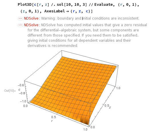
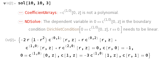
Now I add an axial diffusion term to the PDE, which I match with an outlet condition, i.e. a condition at the z=1 boundary:

sol[Pe_, α_, ω_] := NDSolve[ {r D[c[r, z], {z, 2}] + D[r D[c[r, z], r], r] - 2 r Pe /α (1 - r^2) D[c[r, z], z] == 0, c[r, 0] == -1, (* inlet condition *) 0 == D[c[r, z], r] /. r -> 0, (* no flux at cylinder c[1, z] == -ω D[c[r, z], r] /. r -> 1 (* 'uptake' *), c[r, 1] == 0 (* outlet condition *)}, c, {r, 0, 1}, {z, 0, 1}, SolveDelayed -> True, AccuracyGoal -> 15][[1]] 

The output is:

enter image description here

The output is very similar for an outlet condition of 0 == D[c[r, z], z] /. z -> 1.

I am not sure what is going on here. I believe the last problem is well-posed since I have an outlet condition. Please let me know what your thoughts are, and how to interpret Mathematica's error messages here.

$\endgroup$

1 Answer 1

6
$\begingroup$

OK, figured it out! Mathematica misunderstood my Robin BC as a Dirichlet BC, which is why it gave the above error message. Instead of writing things like c[1, z] == -ω D[c[r, z], r] /. r -> 1 (which Mathematica misinterprets), properly specifying boundary conditions with NeumannValue and DirichletCondition gets the job done.

\[CapitalOmega] := Rectangle[{0, 0}, {Xmax, 1}]; (* RegionPlot[\[CapitalOmega]/.Xmax\[Rule]10, \ AspectRatio\[Rule]Automatic] *) op := Pe Y (1 - Y/2) D[c[X, Y], X] - D[c[X, Y], {Y, 2}] op := Pe Y (1 - Y/2) \!\( \*SubscriptBox[\(\[PartialD]\), \(X\)]\(c[X, Y]\)\) - \!\( \*SubsuperscriptBox[\(\[Del]\), \({X, Y}\), \(2\)]\(c[X, Y]\)\) \[CapitalGamma]N := NeumannValue[-\[Mu]eff c[X, Y], Y == 0] \[CapitalGamma]N2 := NeumannValue[0, X == Xmax] \[CapitalGamma]D1 := DirichletCondition[c[X, Y] == 1, X == 0] \[CapitalGamma]D2 := DirichletCondition[c[X, Y] == 0, X == Xmax] Pe = 10; \[Mu]eff = 10; Xmax = 11; sol = NDSolveValue[{op == \[CapitalGamma]N + \[CapitalGamma]N2, \ \[CapitalGamma]D1 , \[CapitalGamma]D2}, c, {X, Y} \[Element] \[CapitalOmega]] ContourPlot[sol[X, Y], {X, 0, Xmax}, {Y, 0, 1}, Contours -> Table[ci, {ci, 0, 1, 1/20 // N}], AxesLabel -> {X, Y}, AspectRatio -> 0.2, ContourLabels -> True, AxesLabel -> {X, Y}, PlotRange -> All, AspectRatio -> 0.3, PlotLabel -> "Pe = " <> ToString[Pe] <> ", \!\(\*SubscriptBox[\(\[Mu]\), \(eff\)]\) = " <> ToString[\[Mu]eff]] (*Plot3D[sol[X,Y],{X,0,Xmax},{Y,0,1},AxesLabel\[Rule]{X,Y,c}, \ PlotRange\[Rule]All]*) 

I focused on the following similar (but mildly easier) boundary value problem from this paper:
enter image description here

My numerics produced with the above code (left) appears to be a very good match to the published result (right). enter image description here

$\endgroup$

Start asking to get answers

Find the answer to your question by asking.

Ask question

Explore related questions

See similar questions with these tags.