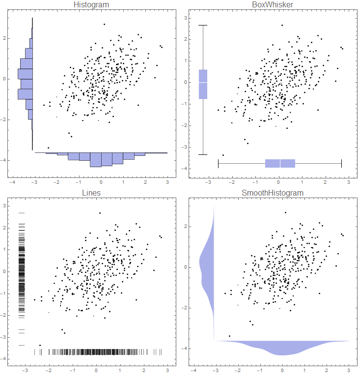
Instead of manually messing with Inset as suggested by m_goldberg, the link supplied by abdullah to the plotGrid function written by Jens did 99% of what I wanted automatically. It only took an If to test if a list element is a Graphics or not to get it to where I wanted. I've also modified the options to allow for internal padding of the figures.
The modified code is below the figures.
e.g.,
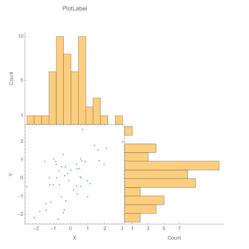
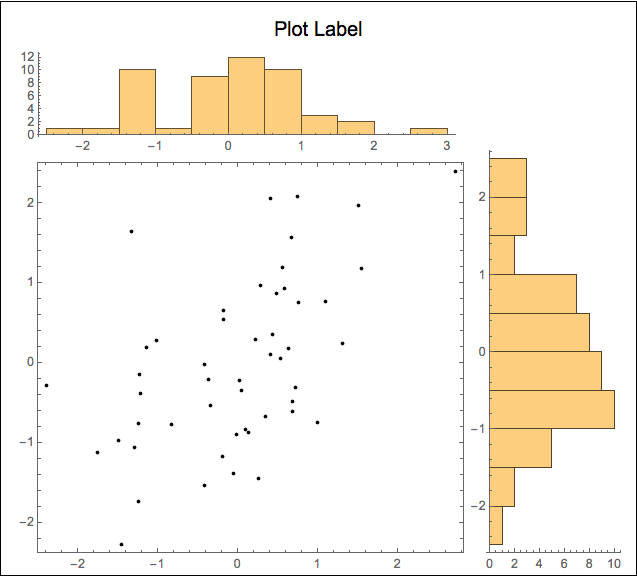
plotGrid[{{histPlot1, None}, {listPlot, histPlot2}}, 500, 500, sidePadding -> 40, internalSidePadding -> 0]
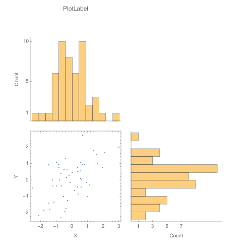
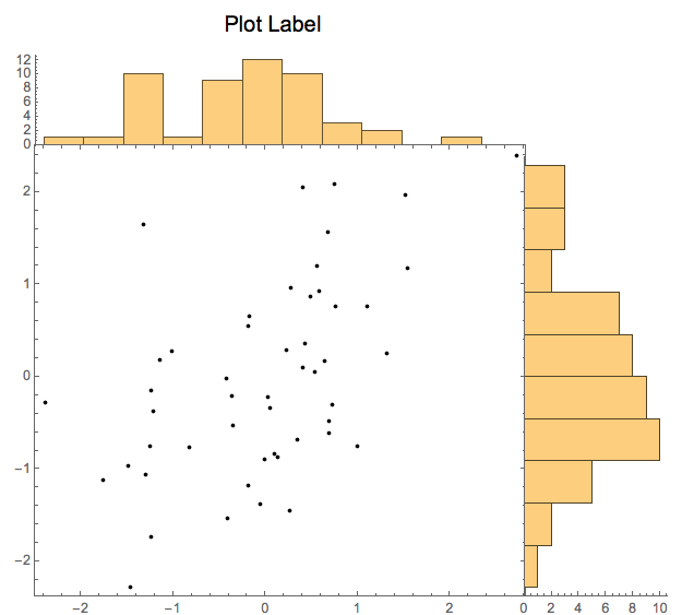
plotGrid[{{histPlot1, None}, {listPlot, histPlot2}}, 500, 500, sidePadding -> 40, internalSidePadding -> 10]
 Clear[plotGrid]
plotGrid::usage = "plotGrid[listOfPlots_, imageWidth_:720, \ imageHeight_:720, Options] creates a grid of plots from the list \ which allows the plots to the same axes with various padding options. \ For an empty cell in the grid use None or Null. Additional options \ are: ImagePadding\[Rule]{{40, 40},{40, 40}}, InternalImagePadding\ \[Rule]{{0, 0},{0, 0}}. ImagePadding can be given as an option for\ the figure as well \nCode modified from: \ https://mathematica.stackexchange.com/questions/6877/do-i-have-to-\ code-each-case-of-this-grid-full-of-plots-separately" Options[plotGrid] = Join[{sidePadding -> {{40, 40}, {40, 40}} , internalSidePadding -> {{0, 0}, {0, 0}} } , Options[Graphics]]; plotGrid[l_List, w_: 720, h_: 720, opts : OptionsPattern[]] := Module[{nx, ny, sidePadding = OptionValue[plotGrid, sidePadding], internalSidePadding = OptionValue[plotGrid, internalSidePadding], topPadding, widths, heights, dimensions, positions, singleGraphic, frameOptions = FilterRules[{opts}, FilterRules[Options[Graphics], Except[{Frame, FrameTicks}]]]}, (*expand [ internal]SidePadding arguments to 4 in case given as single \ argument or in older form of 1 arguments *) Switch[Length[{sidePadding} // Flatten], 2, sidePadding = {{sidePadding[[2]], sidePadding[[2]]}, {sidePadding[[1]], sidePadding[[1]]}}, 4, sidePadding = sidePadding, _, sidePadding = {{sidePadding, sidePadding}, {sidePadding, sidePadding}} ]; Switch[Length[{internalSidePadding} // Flatten], 2, internalSidePadding = {{internalSidePadding[[2]], internalSidePadding[[2]]}, {internalSidePadding[[1]], internalSidePadding[[1]]}}, 4, internalSidePadding = internalSidePadding, _, internalSidePadding = {{internalSidePadding, internalSidePadding}, {internalSidePadding, internalSidePadding}} ]; {ny, nx} = Dimensions[l]; widths = (w - (Plus @@ sidePadding[[1]]))/nx Table[1, {nx}]; widths[[1]] = widths[[1]] + sidePadding[[1, 1]]; widths[[-1]] = widths[[-1]] + sidePadding[[1, 2]]; heights = (h - (Plus @@ sidePadding[[2]]))/ny Table[1, {ny}]; heights[[1]] = heights[[1]] + sidePadding[[2, 1]]; heights[[-1]] = heights[[-1]] + sidePadding[[2, 2]]; positions = Transpose@ Partition[ Tuples[Prepend[Accumulate[Most[#]], 0] & /@ {widths, heights}], ny]; Graphics[Table[ singleGraphic = l[[ny - j + 1, i]]; If[Head[singleGraphic] === Graphics, Inset[Show[singleGraphic, ImagePadding -> ({{If[i == 1, sidePadding[[1, 1]], 0], If[i == nx, sidePadding[[1, 2]], 0]}, {If[j == 1, sidePadding[[2, 1]], 0], If[j == ny, sidePadding[[2, 2]], 0]}} + internalSidePadding), AspectRatio -> Full], positions[[j, i]], {Left, Bottom}, {widths[[i]], heights[[j]]}] ], {i, 1, nx}, {j, 1, ny}], PlotRange -> {{0, w}, {0, h}}, ImageSize -> {w, h}, Evaluate@Apply[Sequence, frameOptions]]]
Graphics[{Inset[histPlot2],...}]. See help forInsetto align properly. $\endgroup$