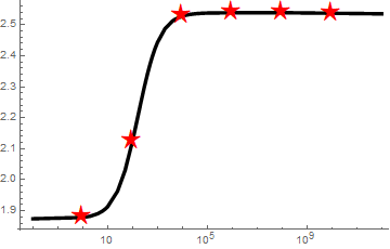
As Henrik Schumacher correctly points out in the comments, the stars on the plot produced by the naive application of the undocumented MeshFunctions -> {"ArcLength"} option
do not look equidistantly spaced with respect to arclength
It took me a while to figure out what happens. The reason is that scales in the vertical and horizontal directions of the plot differ by an order of magnitude. I tried other plotting functions like ListPlot, Plot, ParametricPlot and found that all of them also suffer from this issue.
The following approach solves the problem exactly.
We start by defining our data1:
b1={1.8743,1.8784,1.88248,1.89049,1.89828,1.90587,1.91327,1.96335,2.03035,2.12536,2.23701,2.30098,2.34255,2.37175,2.3934,2.42334,2.44307,2.48725,2.51208,2.5173,2.52799,2.53164,2.53348,2.53533,2.53625,2.53745,2.53793,2.53894,2.53909,2.53543}; ks1={0.01,1.,2.,4.,6.,8.,10.,25.,50.,100.,200.,300.,400.,500.,600.,800.,1000.,2000.,4000.,5000.,10000.,15000.,20000.,30000.,40000.,70000.,100000.,1.*10^6,1.*10^8,1.*10^12}; data1 = Transpose[{ks1, b1}];
Now define future AspectRatio of the plotting area (the option AspectRatio determines the actual aspect ratio of the plotting area with PlotRangePadding included):
aspectRatio = 1./GoldenRatio;
The Graphics produced by ListLogLinearPlot contains log-transformed data plotted in the usual linear cordinate system (it is just Ticks what creates the illusion of a logarithmic coordinate system):
data1Log = {Log@#1, #2} & @@@ data1; dataRange = MinMax /@ Transpose[data1Log];
Now create rescaling function and its inverse:
t = RescalingTransform[ MinMax /@ Transpose[data1Log], {{0, 1}, {0, aspectRatio}}]; tInv = InverseFunction[t];
This function makes vertical and horizontal scales equal in Graphics.
Then we use MeshFunctions -> {"ArcLength"} for generating the equidistantly spaced points with respect to arclength:
s2 = ListLinePlot[t[data1Log], PlotRange -> All, MeshFunctions -> {"ArcLength"}, Mesh -> True];
Extracting the equidistant points and performing the inverse coordinate transform:
pts = tInv @@@ Cases[Normal[s2], _Point, -1];
Now we can use these coordinates for placing the star glyphs in Epilog:
Show[ListLogLinearPlot[data1, Joined -> True, PlotStyle -> {Black, Thickness[0.01]}, AxesStyle -> Black, PlotRange -> All, Epilog -> {Red, Translate[Inset[Style["☆", 15, Bold], {0, 0}], pts]}, AspectRatio -> aspectRatio], PlotRange -> dataRange, PlotRangePadding -> Scaled[.05]]

Note however that Mathematica can't guarantee exact positioning for the font glyphs on the plot. ResourceFunction["PolygonMarker"] guarantees exact positioning of the markers:
Show[ListLogLinearPlot[data1, Joined -> True, PlotStyle -> {Black, Thickness[0.01]}, AxesStyle -> Black, PlotRange -> All, Epilog -> {FaceForm[], EdgeForm[Red], ResourceFunction["PolygonMarker"]["FivePointedStar", Offset[5], pts]}, AspectRatio -> aspectRatio], PlotRange -> dataRange, PlotRangePadding -> Scaled[.05]]
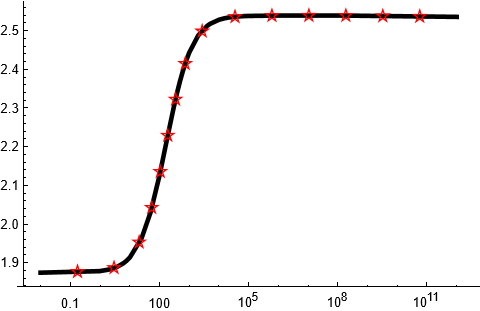
Voila! :)
UPDATE: I just accidentally found that I knew about MeshFunctions -> {"ArcLength"} already several years ago but completely forgot due to non-use of this functionality. I can add to that old post that now we have the wonderful GraphicsInformation function by Carl Woll which simplifies things considerably.