9
$\begingroup$

I've been trying to analyse some SEM images to determine grain areas and sizes. Some of my images (I've attached an example below) appear to have horizontal bands that manifest as regions with different brightness, which leads to discontinuities when detecting via MorphologicalComponents (code snippet below).

I've tried applying a number of filters (Meanfilter, Medianfilter, Gaussianfilter etc.) but haven't been able to come up with a solution for this. Could anyone please help? Thanks.
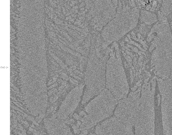
Original image: Original image 
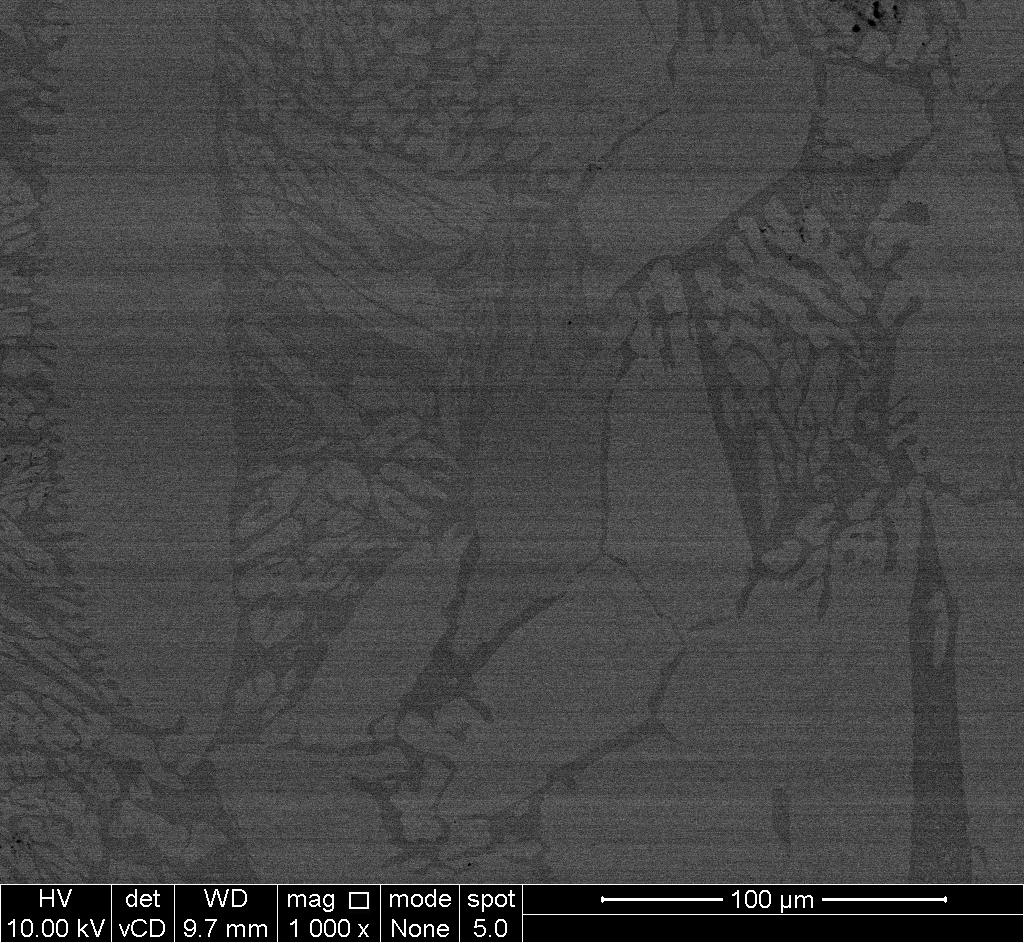
Results after colorising components Colorising components An example of what I hope to get: What I hope to get

data = Import["https://i.sstatic.net/uVv8l.jpg"] snip = ImageTake[data, 880]; ImageHistogram[snip] regions = ColorNegate[Binarize[snip, .283]]; inverse = ColorNegate[%]; medianF = MedianFilter[inverse, 1]; ImageHistogram[medianF] components = MorphologicalComponents[medianF, 0.5, CornerNeighbors -> False]; Colorize[components] masks = ComponentMeasurements[components, "Mask"]; areas = (ComponentMeasurements[masks[[#, 2]], "Area"][[1]][[2]]) & /@Range[1, Length[masks]]; coords = (ComponentMeasurements[masks[[#, 2]],"Centroid"][[1]][[2]]) & /@ Range[1, Length[masks]]; 
$\endgroup$
4
  • $\begingroup$ Does the noise manifest when you take a blank image? If so, you could take a blank image of the noise and subtract that from your images. $\endgroup$ Commented Jun 7, 2019 at 11:01
  • $\begingroup$ Nope, sadly. I took a few images during that run. The last image I've attached in the question is an example of this - and there were no artefacts there. There must have been some fluctuations during the scanning process, maybe because the sample was (somewhat) magnetic. $\endgroup$ Commented Jun 7, 2019 at 11:03
  • 1
    $\begingroup$ Probably overthinking it, but you could transfer learn this U-Net on your working data to segment the image. But more than likely you can just solve this using some smart filtering (have a look at ImagePyramid) $\endgroup$ Commented Jun 7, 2019 at 12:45
  • 1
    $\begingroup$ Just a thought, but you can attempt to model the noise with something like MedianFilter[i, {0, 50}], (across 0 vertical, 50 horizontal pixels) which you could then try to subtract from the image. $\endgroup$ Commented Jun 8, 2019 at 18:42

2 Answers 2

13
$\begingroup$

One thing to look at is to level-adjust each line separately by dividing (or subtracting) the mean of the line's gray value:

img = ImageCrop[ColorConvert[Import["https://i.sstatic.net/uVv8l.jpg"], "Grayscale"], {Full, 850}, {Center, Bottom}]; calib = Rescale[ With[{mean = Mean[#]}, # - mean] & /@ ImageData[img, "Real"] ] // Image 

This removes a good portion of the fluctuations

Mathematica graphics

After that, you can try your smoothing and segmentation again

bin = DeleteSmallComponents[ ColorNegate[MedianFilter[calib, 5]] // Binarize, 100 ]; HighlightImage[calib, bin] 

Mathematica graphics

$\endgroup$
6
$\begingroup$

I like what @halirutan did and had a slight riff on it that appears to yield a better result.

Rescale[With[{meanFiltered = MeanFilter[#, 50]}, # - meanFiltered] & /@ ImageData[img, "Real"]] // Image 

The result of this: Bands removed with MeanFilter radius of 50

If I get time, I might experiment a bit with the "radius" of the MeanFilter to see if that improves the results.

Update: Using Manipulate, it appears that the best results occur between about 50 and 70, after which the banding starts reappearing and is more significant at about 120.

Manipulate[calib = Rescale[With[{meanFiltered = MeanFilter[#, radius]}, # - meanFiltered] & /@ImageData[img, "Real"]] // Image, {{radius, 50}, 10, 250, 5}] 

Update2: I decided to let a program find the optimal by doing this:

initialImageData = ImageData[img, "Real"]; allSortedImages = With[ {choices = Table[Rescale[ With[ {meanFiltered = MeanFilter[#, radius]}, # - meanFiltered ] & /@ initialImageData], {radius, 30, 100, 1}]}, SortBy[choices, Total[initialImageData - #] &] ]; 

That gives this as the best image.

allSortedImages[[1]] // Image 

More optimal choice

I modified this slightly just to more easily be able to find what was the optimal radius.

initialImageData = ImageData[img, "Real"]; allAdjustedImages = Table[Rescale[ With[ {meanFiltered = MeanFilter[#, radius]}, # - meanFiltered ] & /@ initialImageData], {radius, 30, 100, 1}]; allSortedImages = SortBy[allAdjustedImages, Total[initialImageData - #] &]; Position[allAdjustedImages, allSortedImages[[1]]] 

The position returned is 38 (and the image is the same as above).

$\endgroup$
2
  • $\begingroup$ Just for clarity, the position of 38 is a radius of 68. The order of "goodness" based on my crude cost function is the following: {38, 36, 37, 39, 33, 35, 32, 34, 40, 30, 31, 29, 41, 42, 28, 27, 43, \ 44, 26, 45, 25, 46, 17, 18, 19, 20, 24, 23, 47, 16, 15, 22, 21, 14, \ 51, 49, 50, 48, 52, 53, 12, 54, 58, 57, 55, 8, 1, 56, 59, 13, 60, 11, \ 9, 6, 63, 61, 10, 62, 7, 70, 71, 5, 65, 64, 67, 66, 69, 68, 2, 4, 3} $\endgroup$ Commented Jun 10, 2019 at 17:41
  • $\begingroup$ An expert on these sorts of images might benefit by looking at this: Manipulate[ allSortedImages[[i]] // Image, {i, 1, Length[allSortedImages], 1}]. Hit the "play" button on the manipulate and you can see that different filtering brings out different elements. $\endgroup$ Commented Jun 10, 2019 at 18:04

Start asking to get answers

Find the answer to your question by asking.

Ask question

Explore related questions

See similar questions with these tags.