Hi I am new to using Mathematica, so am not too confident. I am essentially trying to model vibrations of a guitar sound board for a project. It would be great to get some visualisations of the eigenfunctions. Apologies if some of the Qs are simple, I am learning as I go.
I started with finding a simplified equation for the guitar outline (sort of avocado shaped).
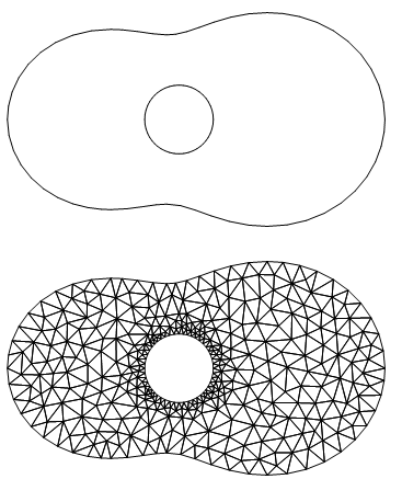
PolarPlot[4 + 1/2*Cos[t] + 3/2*Cos[2*t], {t, 0, 2*Pi}, PlotRange -> {{-6, 6}, {-6, 6}}] I've switched to cartesian coordinates here and included a circle to account for the soundhole.
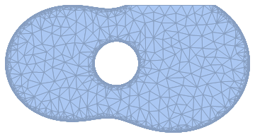
tocartesian = {t -> ArcTan[x, y], r -> Sqrt[x^2 + y^2]} guitarregion = ImplicitRegion[ r < 4 + 1/2*Cos[t] + 3/2*Cos[2*t] /. tocartesian // Simplify, {x, y}] soundholeregion = ImplicitRegion[r < 1 /. tocartesian // Simplify, {x, y}] wholeregion = RegionDifference[guitarregion, soundholeregion] DiscretizeRegion[wholeregion, PrecisionGoal -> 8] RegionMeasure[%] This produces a mesh that is slightly cut off at the top and I am unsure why...
Next, after looking at some other queries on stack exchange I have seen this code utilising the inbuilt functions on Mathematica (Numerically solving Helmholtz equation in 2D for arbitrary shapes):
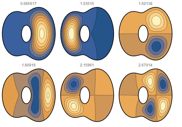
region = {eigenvalues[region], eigenfunctions[region]} = NDEigensystem[{-Laplacian[u[x, y], {x, y}], DirichletCondition[u[x, y] == 0, True]}, u[x, y], {x, y} \[Element] region, 6]; Grid[Partition[ Table[Show[{ContourPlot[ eigenfunctions[region][[j]], {x, y} \[Element] region, Frame -> None, PlotPoints -> 60, PlotRange -> Full, PlotLabel -> eigenvalues[region][[j]]], RegionPlot[region, PlotStyle -> None, BoundaryStyle -> {Black, Thick}]}], {j, 1, Length[eigenvalues[region]]}], 3]] Does this only work for arbitrary/ symmetrical shapes? If I input my region as
region = wholeregion It comes up with the message I should use 'ToElementMesh'. I am quite stuck really as to how to proceed since I don't fully understand the software. Any advice/ information would be really appreciated. Maybe this is just not possible!

