The Discrete System:
$$ \begin{align} x_{n+1}&=c \left(1-(x_n+y_n)\right)+x_n \left(1-p y_n\right)\\ y_{n+1}&=\left(p x_n+b\right)y_n \end{align} $$
The Discrete System code:
F[{x_, y_}, {b_, c_, p_}] := Evaluate[{(1 - p*y)*x + c*(1 - x - y), (p*x + b)*y}] MatrixForm@(F[X, μ]) X = {x, y}; μ = {b, c, p};
The Jacobian Matrix:
J[{x_, y_}, {b_, c_, p_}] := Evaluate@D[F[X, μ], {X}] MatrixForm@(J[X, μ])
The fixed points:
X1[{b_, c_, p_}] = Simplify@SolveValues[F[X, μ] - X == 0, X][[1]]; X2[{b_, c_, p_}] = Simplify@SolveValues[F[X, μ] - X == 0, X][[2]]; MatrixForm@X1[μ] MatrixForm@X2[μ]
Linear approximations:
J1[{b_, c_, p_}] := Evaluate[FullSimplify@J[X1, μ]] J2[{b_, c_, p_}] := Evaluate[FullSimplify@J[X2, μ]] MatrixForm[J1[μ]] J2[{b_, c_, p_}] := Evaluate[FullSimplify@J[X2, μ]] MatrixForm[J1[μ]]
Conditions on the parameters to study the stability of the fixed points:
Local stability of the fixed point $X_{1}$:
Reduce[Tr[J1[μ]] - 1 < Det[J1[μ]] < 1 && Variables[J1[μ]] > 0](*locally stable*) (*Conditions on system parameters*) Reduce[1 < Det[J1[μ]] < Tr[J1[μ]] - 1 && Variables[J1[μ]] > 0](*locally unstable*) (*False*)
Local stability of the fixed point $X_{2}$:
Reduce[Tr[J2[μ]] - 1 < Det[J2[μ]] < 1 && Variables[J2[μ]] > 0](*locally stable*) (*Conditions on system parameters*) Reduce[1 < Det[J2[μ]] < Tr[J2[μ]] - 1 && Variables[J2[μ]] > 0](*locally unstable*) (*Conditions on system parameters*)
Stability test for $X_{1}$ with $b=1/2$, $c=1/100$ and $p=8/10$:
μ0 = {1/2, 1/100, 8/10}; Det[J1[μ0]] Det[J1[μ0]] < 1 Tr[J2[μ0]] - 1 < Det[J2[μ0]] < 1 (*Stability*) (*16781/17000*) (*True*) (*True*)
Stability test for $X_{2}$ with $b=1/2$, $c=1/100$ and $p=8/10$:
μ0 = {1/2, 1/100, 8/10}; Det[J2[μ0]] Det[J2[μ0]] < 1 Tr[J2[μ0]] - 1 < Det[J2[μ0]] < 1 (*Stability*) (*1287/1000*) (*False*) (*False*)
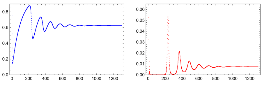
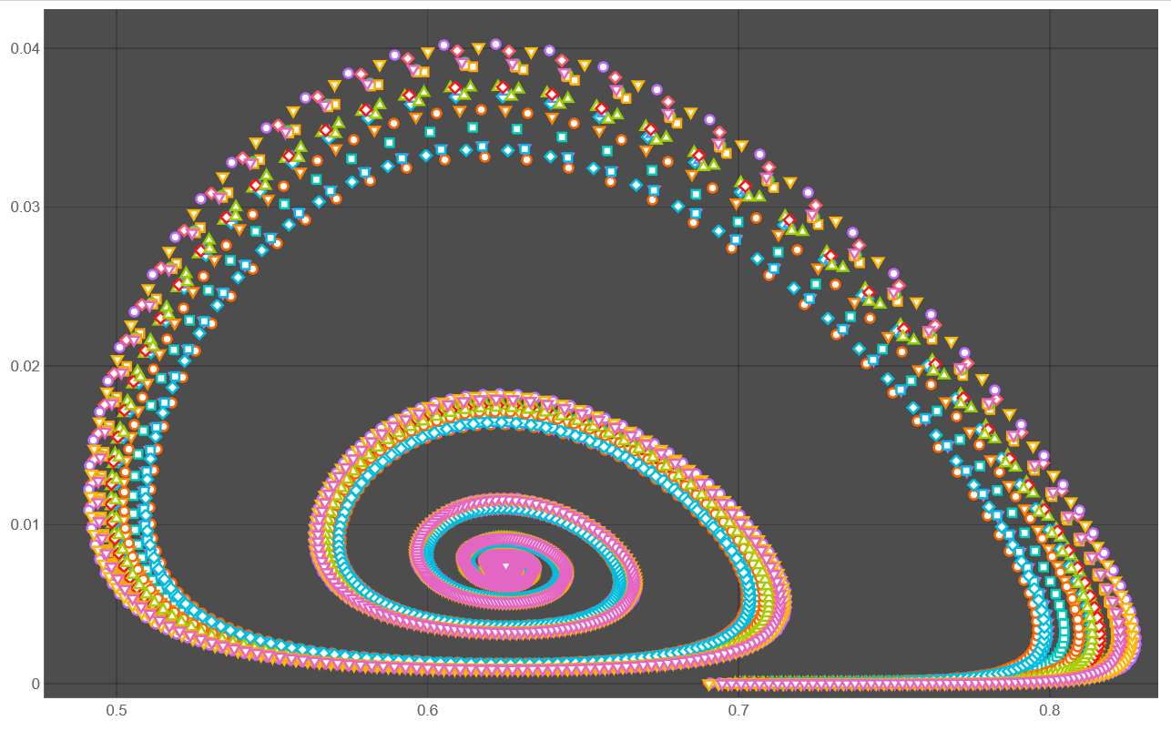
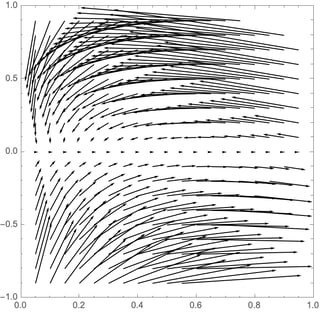
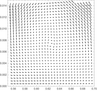
Time Series and Phase Portrait:
Using RecurrenceTable:
data = With[{b = 1/2, c = 1/100, p = 8/10, X0 = {1, 3/10}}, RecurrenceTable[{x[n + 1] == (1 - p*y[n])*x[n] + c*(1 - x[n] - y[n]), y[n + 1] == (p*x[n] + b)*y[n], {x[0], y[0]} == {X0[[1]], X0[[2]]}}, {x, y}, {n, 1, 1300}]];
Time Series:
ListPlot[data[[All, 1]], Frame -> True, FrameStyle -> Black, PlotStyle -> {Blue}, PlotRange -> {All, {0, 0.9}}, AspectRatio -> 1/GoldenRatio] ListPlot[data[[All, 2]], Frame -> True, FrameStyle -> Black, PlotStyle -> {Red}, PlotRange -> {All, {0, 0.065}}, AspectRatio -> 1/GoldenRatio]
Phase Portrait:
ListPlot[data, Frame -> True, FrameStyle -> Black, PlotRange -> {All, {-0.005, 0.11}}, PlotStyle -> Black, AspectRatio -> 1]
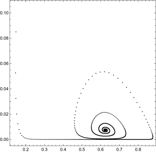
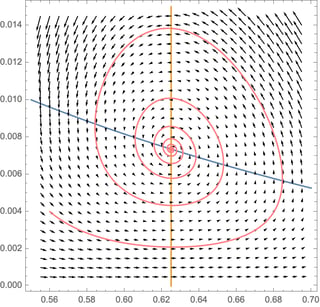
An additional code:
PhasePortrait[data_, linap_, fp_, range_, style_] := Module[{stcond, plot}, stcond[linap2_, fp2_] = Piecewise[{{Graphics[List[PointSize[0.012], Lighter[Blue], Point[fp]]], Tr[linap] - 1 < Det[linap] < 1}, {Graphics[ List[{PointSize[0.012], Black, Point[fp]}, {PointSize[0.006], White, Point[fp]}]], 1 < Det[linap] < Tr[linap] - 1}}]; plot = ListPlot[data, PlotRange -> range, PlotStyle -> style, Frame -> True, FrameStyle -> Black, AspectRatio -> 1, ImageSize -> Medium]; Return[Show[plot, stcond[linap, fp]]]] (*We can improve this code, PRG!*)
Note: If $\text{det}(J(X_{0}))=1$, the fixed point $X_{0}$ can be stable or unstable and, along with other conditions, it can be a Neimark-Sacker bifurcation.
Test:
PhasePortrait[data, J1[μ0], X1[μ0], {All, {-0.005, 0.11}}, Black]
I hope you enjoy it!
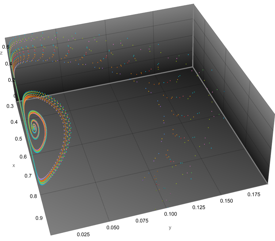
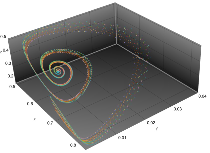
x0,y0,z0,p,b,c. Why do you use 2D subspace to compute Jacobian? $\endgroup$