To solve this problem we can use method of line with handmade discreditation on x as follows:
Clear["Global`*"] Needs["Developer`"] b = -2/3; a = 218; x0 = 0; x1 = 1; u = Exp[-a*(b + t - Log[1 - x])^2]; f[y_] := u /. {t -> 0, x -> y}; f1[y_] := D[u, x] /. {t -> 0, x -> y}; eq = -(1 + x) D[u, t, t] + (1 - 2 x^2)* D[u, x, t] + (1 - x) x^2 D[u, x, x] - 2 x D[u, t] + x (2 - 3 x) D[u, x] // Simplify der[x0_, k_] := NDSolve`FiniteDifferenceDerivative[Derivative[k], x0, "DifferenceOrder" -> "Pseudospectral"]@"DifferentiationMatrix"; Nx = 2^8; II = IdentityMatrix[Nx]; n = Nx - 1; theta = N[Table[i*Pi/n, {i, 0, n}]]; X = N[Chop[((x0 + x1)/2) + ((x0 - x1)/2)*Cos[theta]]]; D1 = der[X, 1]; D2 = der[X, 2]; L1 = (II - 2 DiagonalMatrix[X]^2) . D1; L2 = ((II - DiagonalMatrix[X]) . DiagonalMatrix[X]^2) . D2; L3 = (DiagonalMatrix[X] . (2 II - 3 DiagonalMatrix[X])) . D1; m1 = II + DiagonalMatrix[X]; m2 = 2 DiagonalMatrix[X]; L1 = Developer`ToPackedArray[L1, Real]; L2 = Developer`ToPackedArray[L2, Real]; L3 = Developer`ToPackedArray[L3, Real]; m1 = Developer`ToPackedArray[m1, Real]; m2 = Developer`ToPackedArray[m2, Real]; Psi = Table[Subscript[psi, i][t], {i, Nx}]; Psi1 = Table[Subscript[psi, i]'[t], {i, Nx}]; Pi0 = Table[Subscript[pi, i][t], {i, Nx}]; Pi1 = Table[Subscript[pi, i]'[t], {i, Nx}]; eq1 = -m1 . Pi1 + L1 . Pi0 + L2 . Psi - m2 . Pi0 + L3 . Psi; eq2 = -Psi1 + Pi0; F0 = Chop[f[X] /. Indeterminate -> 0] // Quiet; ic1 = Table[Subscript[psi, i][0] == F0[[i]], {i, Nx}]; F1 = (II - DiagonalMatrix[X]) . Chop[f1[X] /. Indeterminate -> 0] // Quiet; ic2 = Table[Subscript[pi, i][0] == F1[[i]], {i, Nx}]; var = Join[Table[Subscript[psi, i], {i, Nx}], Table[Subscript[pi, i], {i, Nx}]]; sol = NDSolve[Join[Table[eq1[[i]] == 0, {i, Nx}], Table[eq2[[i]] == 0, {i, Nx}], ic1, ic2], var, {t, 0, 1}];
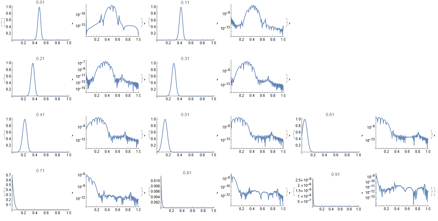
Visualization of solution and absolute error
Table[{ListPlot[Transpose[{X, Psi /. sol[[1]] /. t -> tn}], PlotRange -> All, Joined -> True, PlotLabel -> tn], ListPlot[ Transpose[{X, Abs[(Psi /. sol[[1]] /. t -> tn) - (u /. {t -> tn, x -> X}) // Quiet]}], PlotRange -> All, Joined -> True, ScalingFunctions -> "Log"]}, {tn, 0.01, .91, .1}]
Update 1. We also can implement Runge-Kutta method from my answer here as follows
Clear["Global`*"] Needs["Developer`"] b = -2/3; a = 218; x0 = 0; x1 = 1; u = Exp[-a*(b + t - Log[1 - x])^2]; f[y_] := u /. {t -> 0, x -> y}; f1[y_] := D[u, x] /. {t -> 0, x -> y}; eq = -(1 + x) D[u, t, t] + (1 - 2 x^2)* D[u, x, t] + (1 - x) x^2 D[u, x, x] - 2 x D[u, t] + x (2 - 3 x) D[u, x] // Simplify der[x0_, k_] := NDSolve`FiniteDifferenceDerivative[Derivative[k], x0, "DifferenceOrder" -> "Pseudospectral"]@"DifferentiationMatrix"; Nx = 2^8; II = IdentityMatrix[Nx]; n = Nx - 1; theta = N[Table[i*Pi/n, {i, 0, n}]]; X = N[Chop[((x0 + x1)/2) + ((x0 - x1)/2)*Cos[theta]]]; D1 = der[X, 1]; D2 = der[X, 2]; L1 = (II - 2 DiagonalMatrix[X]^2) . D1; L2 = ((II - DiagonalMatrix[X]) . DiagonalMatrix[X]^2) . D2; L3 = (DiagonalMatrix[X] . (2 II - 3 DiagonalMatrix[X])) . D1; m1 = II + DiagonalMatrix[X]; m2 = 2 DiagonalMatrix[X]; L1 = Developer`ToPackedArray[L1, Real]; L2 = Developer`ToPackedArray[L2, Real]; L3 = Developer`ToPackedArray[L3, Real]; m1 = Developer`ToPackedArray[m1, Real]; m2 = Developer`ToPackedArray[m2, Real]; F0 = Chop[f[X] /. Indeterminate -> 0] // Quiet; F1 = (II - DiagonalMatrix[X]) . Chop[f1[X] /. Indeterminate -> 0] // Quiet; z = ConstantArray[0, 2 Nx]; ff[t_, z_] := Join[Drop[z, Nx], Inverse[m1] . (L1 . Drop[z, Nx] + L2 . Drop[z, -Nx] - m2 . Drop[z, Nx] + L3 . Drop[z, -Nx])]; rk2[ff_, h_][{t_, x_}] := Module[{k1, k2}, k1 = ff[t, x]; k2 = ff[t + h/2, x + h k1/2]; {t + h, x + h k2}] tf = 1; dt = 1/1000; sol = NestList[rk2[ff, dt], {0, Join[F0, F1]}, Round[tf/dt]];
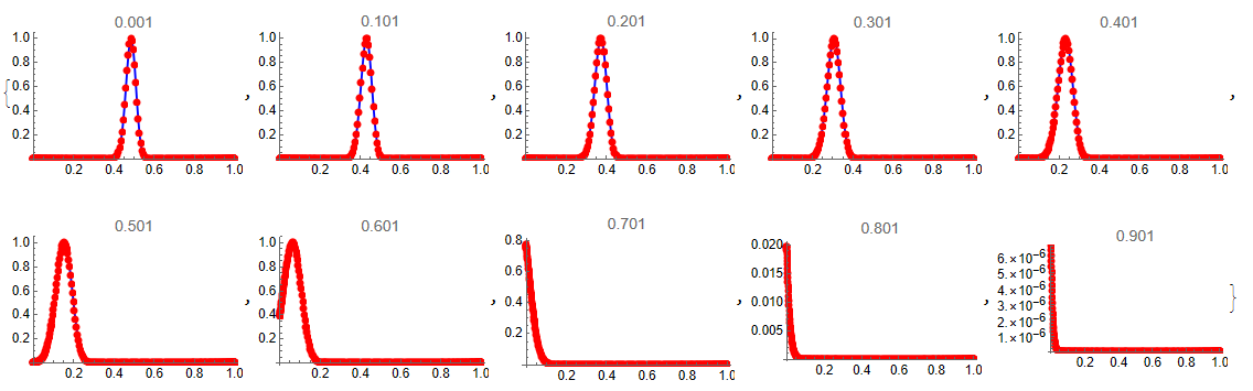
Visualization of numerical solution (red points) and exact solution (blue lines) at different times (shown above)
Table[Show[ ListLinePlot[Transpose[{X, (u /. {t -> i dt, x -> X}) // Quiet}], PlotStyle -> Blue, PlotRange -> All, PlotLabel -> N[i dt]], ListPlot[Transpose[{X, Drop[sol[[i + 1, 2]], -Nx]}], PlotStyle -> Red, PlotMarkers -> {Automatic, Smaller}]], {i, 1, Round[tf/dt], 100}]
DChange[]? It might work on this. $\endgroup$xandbc? $\endgroup$bcwithiconly? $\endgroup$NDSolve? Is it for didactic purposes? $\endgroup$