I'm trying to create a disk with a radial gradient. I found the built in function "RadialGradientFilling" which should do the trick but, alas, I am using an older version of Mathematica where it is not supported. Is there any work around to be able to do something along the lines of
Graphics[{RadialGradientFilling[{Red, Blue}], Disk[]}] in Mathematica 11.1? I know its possible to make a grid of points with some color distribution but I really need it to be applied to a Disk graphic. Any thoughts?
The actual code I'm working on can be found down below. I'm trying to give the gradient color to the yellow Graphic
Manipulate[ Module[{npoints = 2000, munit = 10^11, plotsize = 10, sec2rad = Pi/(180. 3600.), sxy}, imagePos[sourcexy_, mass_, distlens_] := Module[{g = 6.6726*10^-11(*m^3/(kg s^2)*), c = 2.99792458*10^8(*m/ s*), msun = 1.989*10^30(*kg*), parsec = 3.0856*10^16(*m*), ly = 3.26(*parsec*), ds, dl, b, bx, by, u, t1, t2, image1, image2, images}, b = Sqrt[Total[sourcexy^2]]; If[b > 10^-10, ds = 1 parsec 10^9; dl = (distlens parsec 10^9)/ly; u = 4 msun Abs[ds - dl]/(ds dl) (g mass)/c^2; t1 = (1 + Sqrt[1 + (4 u)/b^2])/2; t2 = (1 - Sqrt[1 + (4 u)/b^2])/2, t1 = 0; t2 = 0]; image1 = t1 sourcexy; image2 = t2 sourcexy; images = Join[List[image1], List[image2]]; Return[images]]; source[center_, r_, npoints_] := Module[{p, x, y, points}, p = Table[(2 Pi)/npoints i, {i, 0, npoints}]; x = List[center[[1]] + List[r Cos[p]]]; y = List[center[[2]] + List[r Sin[p]]]; points = MapThread[List, Flatten[List[x, y], 2]]; Return[points]]; If[Sqrt[sourcexy[[1]]^2 + sourcexy[[2]]^2] > 10^-4, sxy = sourcexy, sxy = {0, 0}]; If[Sqrt[sxy[[1]]^2 + sxy[[2]]^2] > r, Graphics[ {{Yellow, Polygon[Part[ Flatten[1/ sec2rad (imagePos[#, munit mass, dl] & /@ source[sec2rad sxy, sec2rad r, npoints]), 1], Table[i, {i, 1, 2 npoints - 1, 2}]]]}, {Yellow, Polygon[Part[ Flatten[1/ sec2rad (imagePos[#, munit mass, dl] & /@ source[sec2rad sxy, sec2rad r, npoints]), 1], Table[i, {i, 2, 2 npoints, 2}]]]}, {Gray, Disk[{0, 0}, plotsize/30]}, Text["source-lens separation (arcsec):" PaddedForm[Sqrt[ sxy[[1]]^2 + sxy[[2]]^2], {4, 2}], {-.06 plotsize, 5/6 plotsize + .5}]}, PlotRange -> plotsize, Frame -> True, ImageSize -> {400, 400}], Graphics[{{Yellow, Polygon[Part[ Flatten[1/ sec2rad (imagePos[#, munit mass, dl] & /@ source[sec2rad sxy, sec2rad r, npoints]), 1], Table[i, {i, 1, 2 npoints - 1, 2}]]]}, {White, Polygon[Part[ Flatten[1/ sec2rad (imagePos[#, munit mass, dl] & /@ source[sec2rad sxy, sec2rad r, npoints]), 1], Table[i, {i, 2, 2 npoints, 2}]]]}, {Gray, Disk[{0, 0}, plotsize/30]}, Text["source-lens separation (arcseconds):" PaddedForm[Sqrt[ sxy[[1]]^2 + sxy[[2]]^2], {4, 2}], {-.06 plotsize, 5/6 plotsize + .5}]}, PlotRange -> plotsize, Frame -> True, ImageSize -> {400, 400}]]], {{sourcexy, {0, 0}}, {-10, -10}, {10, 10}, Locator}, "distance to lens in \!\(\*SuperscriptBox[\(10\), \(9\)]\) light \ years", {{dl, 1.5, ""}, 0.4, 3, Appearance -> "Labeled"}, "radius of circular image in arcsec", {{r, 1, ""}, 0.1, 2, Appearance -> "Labeled"}, "mass of lens in \!\(\*SuperscriptBox[\(10\), \(11\)]\) solar \ masses", {{mass, 10, ""}, 0.1, 100, Appearance -> "Labeled"}, TrackedSymbols :> {sourcexy, dl, r, mass}]