Since the question isn't clear about which datasets are which and arguably has too many parameters, I'll use the example from here instead:
$$ \begin{array}{l} A+B\underset{k_2}{\overset{k_1}{\leftrightharpoons }}X \\ X+B\overset{k_3}{\longrightarrow }\text{products} \\ \end{array} \Bigg\} \Longrightarrow A+2B\longrightarrow \text{products} $$
We solve the system and generate some fake data:
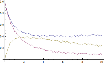
sol = ParametricNDSolveValue[{ a'[t] == -k1 a[t] b[t] + k2 x[t], a[0] == 1, b'[t] == -k1 a[t] b[t] + k2 x[t] - k3 b[t] x[t], b[0] == 1, x'[t] == k1 a[t] b[t] - k2 x[t] - k3 b[t] x[t], x[0] == 0 }, {a, b, x}, {t, 0, 10}, {k1, k2, k3} ]; abscissae = Range[0., 10., 0.1]; ordinates = With[{k1 = 0.85, k2 = 0.15, k3 = 0.50}, Through[sol[k1, k2, k3][abscissae], List] ]; data = ordinates + RandomVariate[NormalDistribution[0, 0.1^2], Dimensions[ordinates]]; ListLinePlot[data, DataRange -> {0, 10}, PlotRange -> All, AxesOrigin -> {0, 0}] The data look like this, where blue is A, purple is B, and gold is X:
The key to the exercise, of course, is the simultaneous fitting of all three datasets in order for the rate constants to be determined self-consistently. To achieve this we have to prepend to each point a number, i, that labels the dataset:
transformedData = { ConstantArray[Range@Length[ordinates], Length[abscissae]] // Transpose, ConstantArray[abscissae, Length[ordinates]], data } ~Flatten~ {{2, 3}, {1}}; We also need a model that returns the values for either A, B, or X depending on the value of i:
model[k1_, k2_, k3_][i_, t_] := Through[sol[k1, k2, k3][t], List][[i]] /; And @@ NumericQ /@ {k1, k2, k3, i, t}; The fitting is now straightforward. Although it will help if reasonable initial values are given, this is not strictly necessary here:
fit = NonlinearModelFit[ transformedData, model[k1, k2, k3][i, t], {k1, k2, k3}, {i, t} ]; 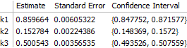
The result is correct. Worth noting, however, is that the off-diagonal elements of the correlation matrix are quite large:
fit["CorrelationMatrix"] (* -> {{ 1., 0.764364, -0.101037}, { 0.764364, 1., -0.376295}, {-0.101037, -0.376295, 1. }} *) Just to be sure of having directly addressed the question, I will note that the process does not change if we have less than the complete dataset available (although the parameters might be determined with reduced accuracy in this case). Typically it will be most difficult experimentally to measure the intermediate, so let's get rid of the dataset for X (i == 3) and try again:
reducedData = DeleteCases[transformedData, {3, __}]; fit2 = NonlinearModelFit[ reducedData, model[k1, k2, k3][i, t], {k1, k2, k3}, {i, t} ]; The main consequence is that the error on $k_3$ is significantly larger:
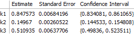
This can be seen to be the result of greater correlation between $k_1$ and $k_3$ when fewer data are available for fitting:
fit2["CorrelationMatrix"] (* -> {{ 1., 0.7390200, -0.1949590}, { 0.7390200, 1., 0.0435416}, {-0.1949590, 0.0435416, 1. }} *) On the other hand, the correlation between $k_2$ and $k_3$ is greatly reduced, so that all of the rate constants are still sufficiently well determined and the overall result does not change substantially.