The hypothesis to test is:
$H_0$: $D$ and $D'$ are random draws from the same population.
$H_1$: The population from which $D$ was drawn is not the same population from which $D'$ was drawn.
A possible approach
Here I modify the notation so that $D \in \{0,1\}^{n \times k}$ and $D' \in \{0,1\}^{m \times k}$.
Combine $D$ and $D'$, then partition the observations in $k$ different ways, each corresponding to the presence of the $i^{\text{th}}$ trait, with $i\in\{1...k\}$. Given $H_0$, the number of observations from $D'$ in the partition with the $i^{\text{th}}$ trait should follow the hypergeometric distribution with PMF:
$$p(a'_i|m,n,a_i)=\frac{\binom{m}{a'_i}\binom{n}{a_i}}{\binom{m+n}{a_i+a'_i}}$$ where $a_i$ and $a'_i$ are the total number of observations in $D$ and $D'$ with the $i^{\text{th}}$ trait.
Further, if $S_i=U(F(a'_i-1;m,n,a_i),F(a'_i;m,n,a_i))$, then $S_i\sim{U(0,1)}$, again assuming $H_0$. Test for $H_0$ by testing if $S\sim{U(0,1)}$, using, e.g., Kolmogorov-Smirnov (which may require relaxing the requirement of independence between the $S_i$).
Demonstrating in R:
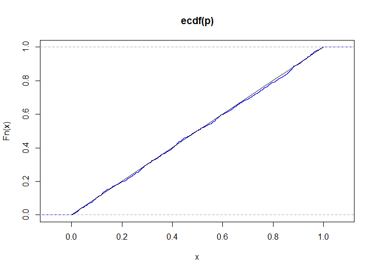
set.seed(704776517) n <- 100L m <- 40L k <- 9L # simulate 1000 KS p-values for identically distributed observations p <- replicate( 1e3, { x <- mapply(\(p) rbinom(n, 1, p), seq(0.1, 0.9, length.out = k)) y <- mapply(\(p) rbinom(m, 1, p), seq(0.1, 0.9, length.out = k)) csy <- colSums(y) csxy <- colSums(x) + csy S <- sapply(1:k, \(i) runif(1, phyper(csy[i] - 1, m, n, csxy[i]), phyper(csy[i], m, n, csxy[i]))) ks.test(S, punif)$p.value } ) plot(ecdf(p), col = "blue") lines(0:1, 0:1)
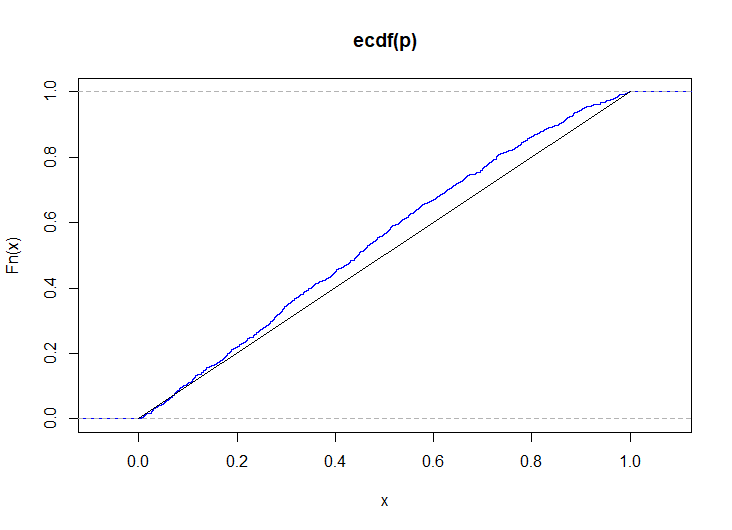
# simulate p-values when the distributions are slightly different p <- replicate( 1e3, { x <- mapply(\(p) rbinom(n, 1, p), seq(0.1, 0.9, length.out = k)) y <- mapply(\(p) rbinom(m, 1, p), seq(0.2, 0.8, length.out = k)) csy <- colSums(y) csxy <- colSums(x) + csy S <- sapply(1:k, \(i) runif(1, phyper(csy[i] - 1, m, n, csxy[i]), phyper(csy[i], m, n, csxy[i]))) ks.test(S, punif)$p.value } ) plot(ecdf(p), col = "blue") lines(0:1, 0:1)
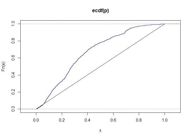
# simulate p-values when the distributions are even more different p <- replicate( 1e3, { x <- mapply(\(p) rbinom(n, 1, p), seq(0.1, 0.9, length.out = k)) y <- mapply(\(p) rbinom(m, 1, p), seq(0.3, 0.7, length.out = k)) csy <- colSums(y) csxy <- colSums(x) + csy S <- sapply(1:k, \(i) runif(1, phyper(csy[i] - 1, m, n, csxy[i]), phyper(csy[i], m, n, csxy[i]))) ks.test(S, punif)$p.value } ) plot(ecdf(p), col = "blue") lines(0:1, 0:1)
The final demonstration is in log-space, so as to test if $S\sim\text{exp}(1)$. (This formulation is not actually needed here, but it demonstrates how to maintain numeric stability if the proportion of observations of $D$ or $D'$ in the partition is very unbalanced).
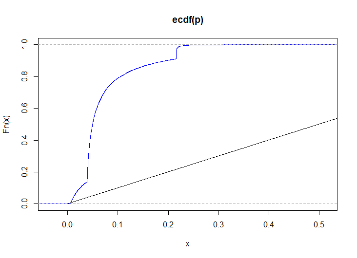
# simulate p-values when the distributions are very different p <- replicate( 1e4, { x <- mapply(\(p) rbinom(n, 1, p), seq(0.1, 0.9, length.out = k)) y <- mapply(\(p) rbinom(m, 1, p), seq(0.7, 0.3, length.out = k)) csy <- colSums(y) csxy <- colSums(x) + csy S <- sapply(1:k, \(i) (a <- -phyper(csy[i], m, n, csxy[i], log.p = TRUE)) - log1p(runif(1)*expm1(phyper(csy[i] - 1, m, n, csxy[i], log.p = TRUE) + a))) ks.test(S, pexp)$p.value } ) plot(ecdf(p), col = "blue") lines(0:1, 0:1)