CLASSIFICATION METHODS IN DATA MINING AND MODELING

DATA MINING AND MODELING UNIT IV CLASSIFICATION

CLASSIFICATION:  Classification is a supervised learning technique used in data mining and machine learning to categorize data into predefined classes or groups based on input features.  In classification, the algorithm learns from a training dataset (where the class labels are already known) and builds a model. This model is then used to predict the class labels of new, unseen data. Example 1: Email Classification Problem: Classify emails as “Spam” or “Not Spam”. Input Attributes: Keywords in the email, sender address, subject line, frequency of certain words, etc. Classes:  Class 1 → Spam  Class 2 → Not Spam Algorithm Used: Naive Bayes classifier or Decision Tree Example 2: Medical Diagnosis Problem: Predict whether a patient has Diabetes or No Diabetes. Input Attributes: Age, BMI, blood pressure, glucose level, insulin level, etc. Classes:  Class 1 → Diabetic  Class 2 → Non-diabetic Algorithm Used: Logistic Regression, Support Vector Machine (SVM) If glucose level and BMI are high, the model might predict the patient as Diabetic.

Predefined Dataset A predefined dataset means a set of data that already has known answers or labels. In this dataset, each record has: •Input data (features) → what we use to make a decision •Output label (class) → the correct answer Because the answers are already known, we can train the computer (model) to learn from it. This is used in supervised learning. Student Marks Attendance Result A 85 90 Pass B 40 50 Fail C 78 80 Pass Example 1: Student Result Prediction

Decision Tree Induction Introduction: Decision Tree Induction is a classification method used to predict the class label of data by learning simple decision rules inferred from the data features. It represents decisions in the form of a tree structure, where: •Each internal node represents a test on an attribute, •Each branch represents the outcome of the test, and •Each leaf node represents a class label (decision or output). Weather Temperature Play Sunny Hot No Sunny Mild Yes Rainy Mild Yes Rainy Cold No

Steps in Decision Tree Induction 1.Select Attribute for Root Node Choose the attribute that best separates the data (using Information Gain, Gain Ratio, or Gini Index). 2.Split Data into Subsets Based on the selected attribute’s possible values. 3.Repeat for Each Subset Continue the process recursively until all data belong to a single class or other stopping conditions are met. 4.Form the Final Decision Tree Important Terms •Information Gain: Measures how much information an attribute gives about the class. Formula: •Entropy: Measures impurity or randomness in data. •Gini Index: Another measure of impurity used in CART (Classification and Regression Trees).

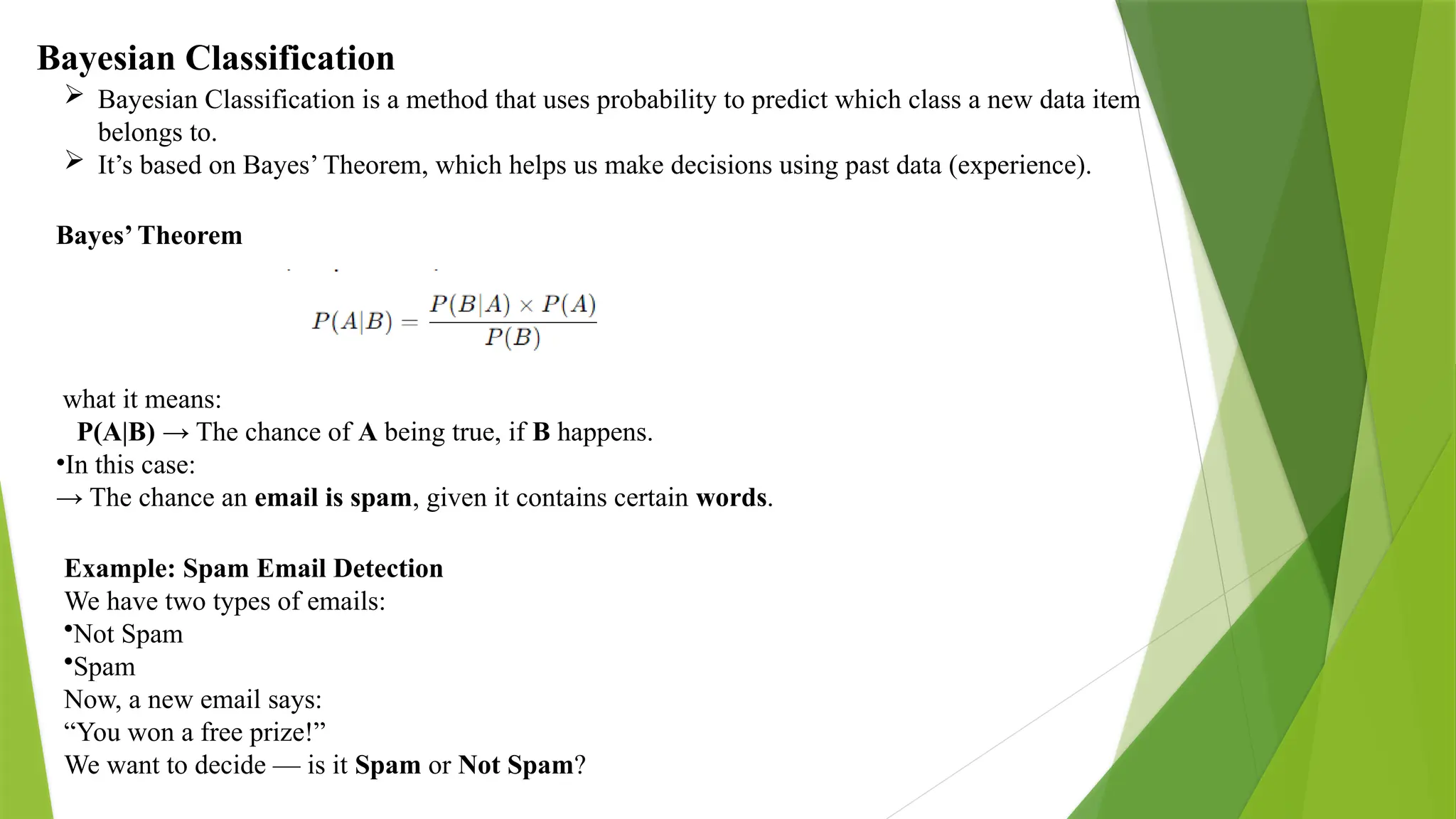
Bayesian Classification  Bayesian Classification is a method that uses probability to predict which class a new data item belongs to.  It’s based on Bayes’ Theorem, which helps us make decisions using past data (experience). Bayes’ Theorem what it means: P(A|B) → The chance of A being true, if B happens. •In this case: → The chance an email is spam, given it contains certain words. Example: Spam Email Detection We have two types of emails: •Not Spam •Spam Now, a new email says: “You won a free prize!” We want to decide — is it Spam or Not Spam?

Step 1: Learn from training data We look at old emails: Contains “Free”? Contains “Prize”? Class Yes Yes Spam Yes No Spam No Yes Not Spam No No Not Spam From this, the computer learns: •Most spam emails contain “Free” or “Prize”. Non-spam emails usually don’t. Step 2: Predict for new email For the new email (“Free Prize”): It checks how often “Free” and “Prize” appear in spam vs. not spam. Then it calculates which is more likely. It finds: Probability(Spam) = higher Probability(Not Spam) = lower Result: It says the new email is Spam.

Rule-Based Classification •Rule-Based Classification is a method of classifying data using IF–THEN rules. •These rules are used to predict the class of new data based on conditions. •It is easy to understand and interpretable, which makes it popular in data mining. What is a Rule? A rule has two parts: IF (Condition) – based on attribute values THEN (Class) – the result or prediction Example: IF outlook = sunny AND humidity = high THEN play = no This means: If the weather is sunny and humidity is high, we do not play. How It Works 1.Generate rules from training data. 2.Evaluate the rules using accuracy or confidence. 3.Apply the best-matching rule to classify new data.

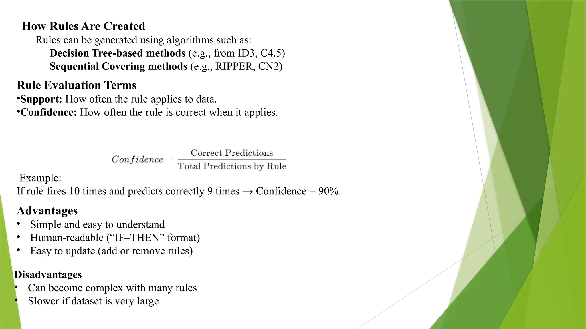
How Rules Are Created Rules can be generated using algorithms such as: Decision Tree-based methods (e.g., from ID3, C4.5) Sequential Covering methods (e.g., RIPPER, CN2) Rule Evaluation Terms •Support: How often the rule applies to data. •Confidence: How often the rule is correct when it applies. Example: If rule fires 10 times and predicts correctly 9 times → Confidence = 90%. Advantages • Simple and easy to understand • Human-readable (“IF–THEN” format) • Easy to update (add or remove rules) Disadvantages • Can become complex with many rules • Slower if dataset is very large

Neural Network 1. Introduction • A Neural Network is a machine learning model inspired by the human brain. • It is made up of small processing units called neurons, which work together to recognize patterns and make predictions. • Used for classification, prediction, pattern recognition, and image processing. 2. Structure of a Neural Network A neural network has layers of neurons: Layer Description Input Layer Takes input features (like data attributes) Hidden Layers Process data through weighted connections Output Layer Gives the final result (class or value) 3.Example (Simple Classification) Imagine we want to predict if a student passes or fails based on: •Hours studied •Attendance

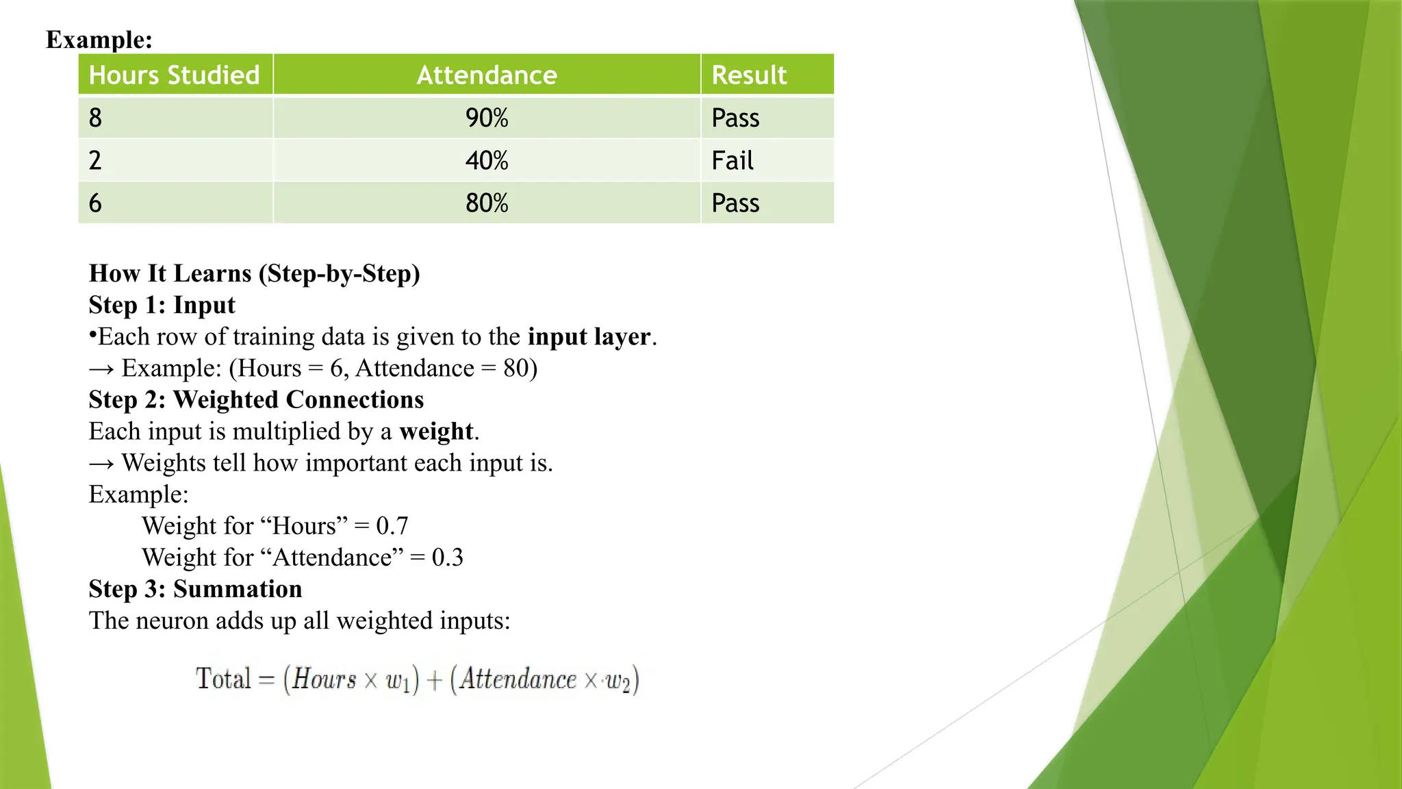
Example: Hours Studied Attendance Result 8 90% Pass 2 40% Fail 6 80% Pass How It Learns (Step-by-Step) Step 1: Input •Each row of training data is given to the input layer. → Example: (Hours = 6, Attendance = 80) Step 2: Weighted Connections Each input is multiplied by a weight. → Weights tell how important each input is. Example: Weight for “Hours” = 0.7 Weight for “Attendance” = 0.3 Step 3: Summation The neuron adds up all weighted inputs:

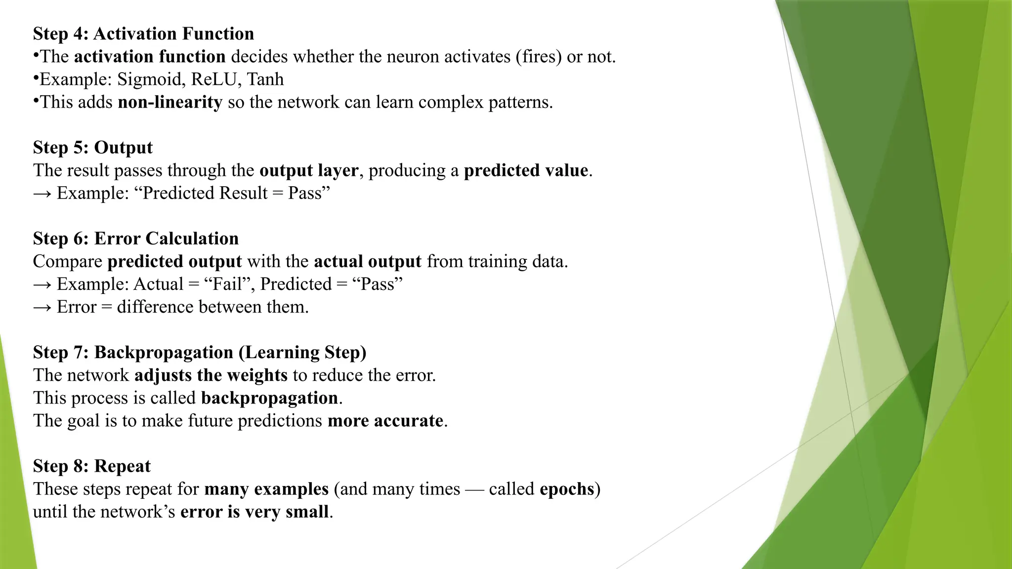
Step 4: Activation Function •The activation function decides whether the neuron activates (fires) or not. •Example: Sigmoid, ReLU, Tanh •This adds non-linearity so the network can learn complex patterns. Step 5: Output The result passes through the output layer, producing a predicted value. → Example: “Predicted Result = Pass” Step 6: Error Calculation Compare predicted output with the actual output from training data. → Example: Actual = “Fail”, Predicted = “Pass” → Error = difference between them. Step 7: Backpropagation (Learning Step) The network adjusts the weights to reduce the error. This process is called backpropagation. The goal is to make future predictions more accurate. Step 8: Repeat These steps repeat for many examples (and many times — called epochs) until the network’s error is very small.

4. After Training Once the neural network has trained: •Now, it can predict new unseen data correctly. Example: New input: Hours = 7, Attendance = 85 Neural Network predicts → “Pass” •It remembers the learned weights. 5. Advantages •Learns complex patterns •Works well with big data •Can handle images, sound, text, etc 6. Disadvantages •Needs a lot of data •Takes time to train

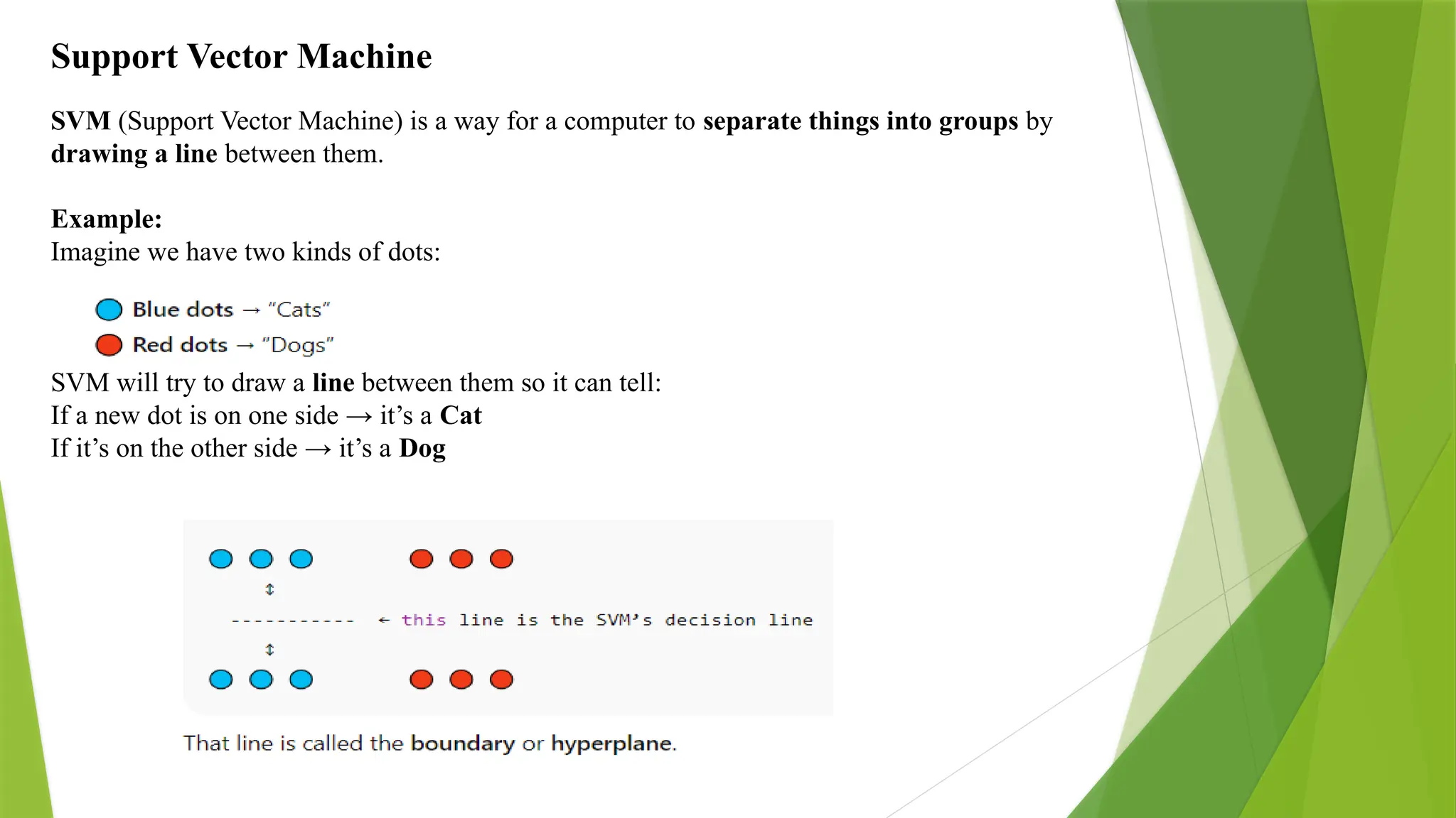
Support Vector Machine SVM (Support Vector Machine) is a way for a computer to separate things into groups by drawing a line between them. Example: Imagine we have two kinds of dots: SVM will try to draw a line between them so it can tell: If a new dot is on one side → it’s a Cat If it’s on the other side → it’s a Dog

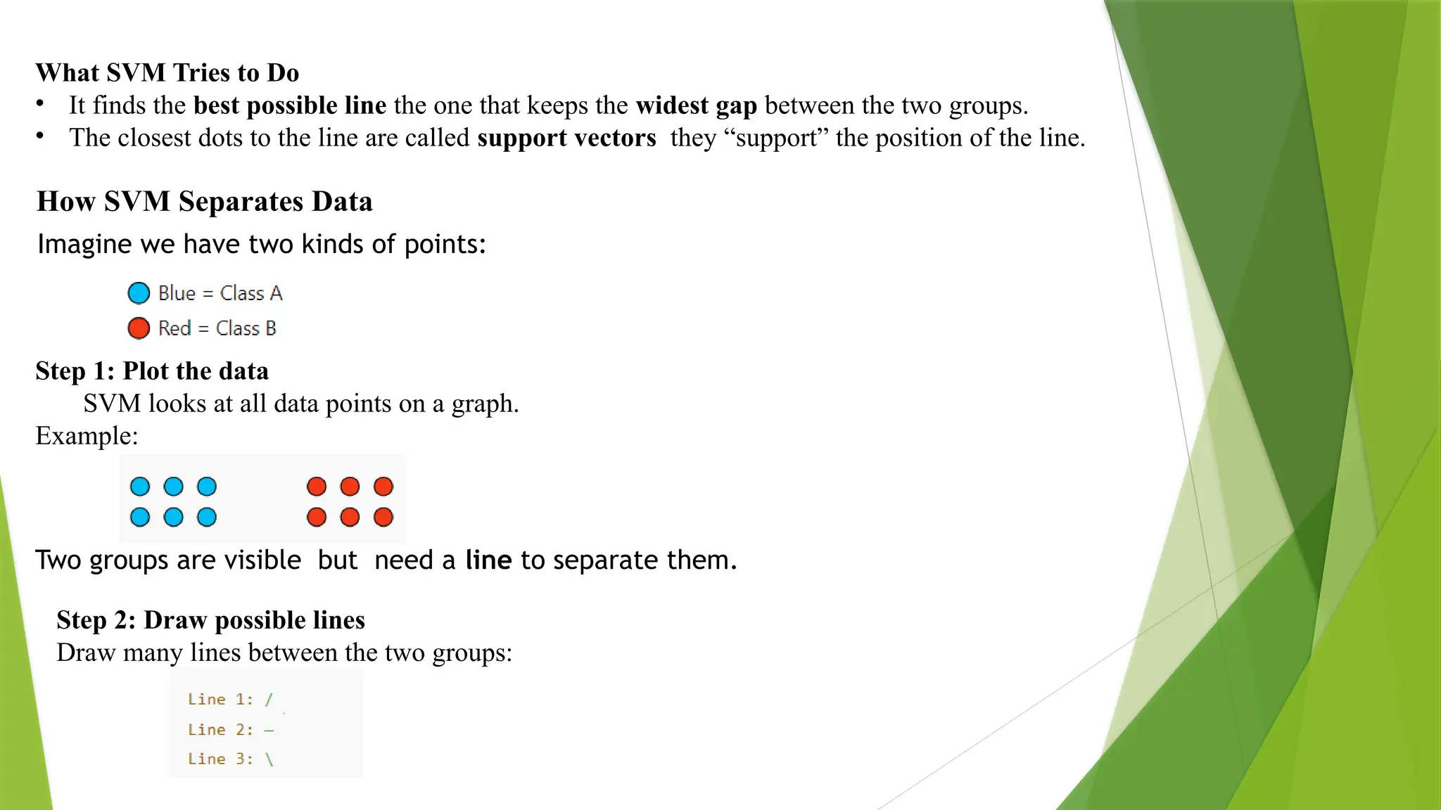
What SVM Tries to Do • It finds the best possible line the one that keeps the widest gap between the two groups. • The closest dots to the line are called support vectors they “support” the position of the line. How SVM Separates Data Imagine we have two kinds of points: Step 1: Plot the data SVM looks at all data points on a graph. Example: Two groups are visible but need a line to separate them. Step 2: Draw possible lines Draw many lines between the two groups:

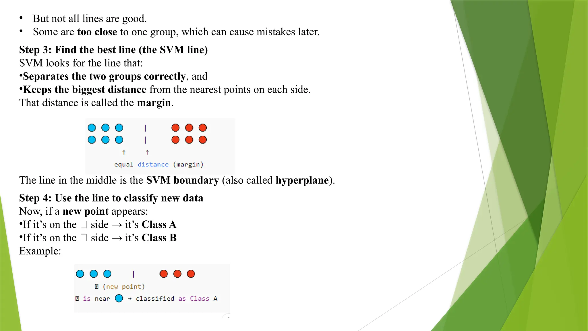
• But not all lines are good. • Some are too close to one group, which can cause mistakes later. Step 3: Find the best line (the SVM line) SVM looks for the line that: •Separates the two groups correctly, and •Keeps the biggest distance from the nearest points on each side. That distance is called the margin. The line in the middle is the SVM boundary (also called hyperplane). Step 4: Use the line to classify new data Now, if a new point appears: •If it’s on the 🔵 side → it’s Class A •If it’s on the 🔴 side → it’s Class B Example:

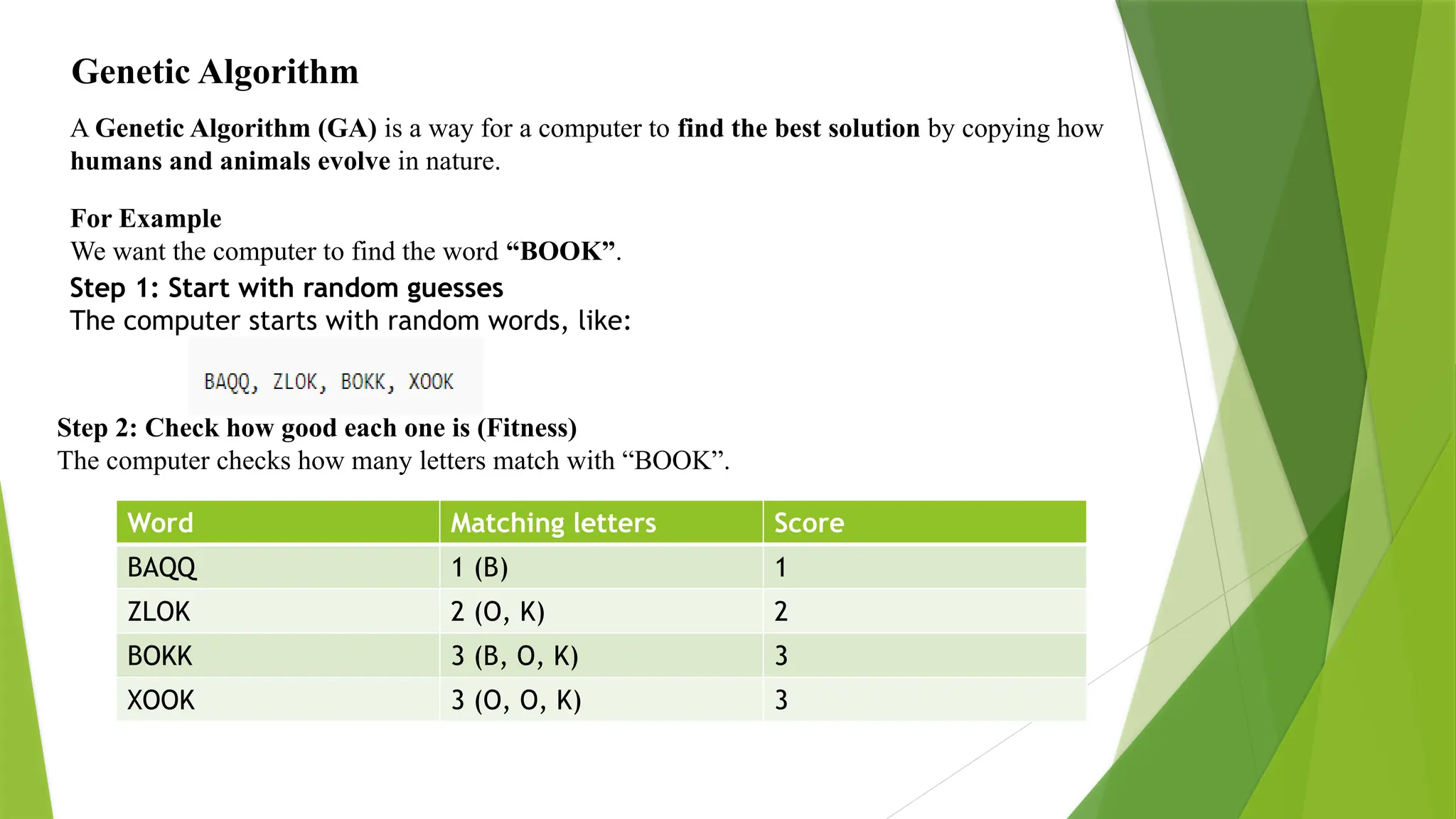
Genetic Algorithm A Genetic Algorithm (GA) is a way for a computer to find the best solution by copying how humans and animals evolve in nature. For Example We want the computer to find the word “BOOK”. Step 1: Start with random guesses The computer starts with random words, like: Step 2: Check how good each one is (Fitness) The computer checks how many letters match with “BOOK”. Word Matching letters Score BAQQ 1 (B) 1 ZLOK 2 (O, K) 2 BOKK 3 (B, O, K) 3 XOOK 3 (O, O, K) 3

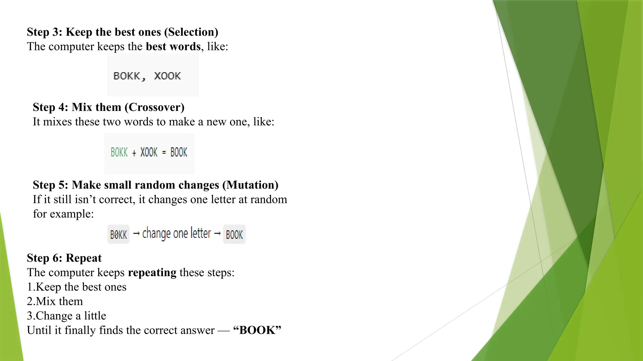
Step 3: Keep the best ones (Selection) The computer keeps the best words, like: Step 4: Mix them (Crossover) It mixes these two words to make a new one, like: Step 5: Make small random changes (Mutation) If it still isn’t correct, it changes one letter at random for example: Step 6: Repeat The computer keeps repeating these steps: 1.Keep the best ones 2.Mix them 3.Change a little Until it finally finds the correct answer — “BOOK”

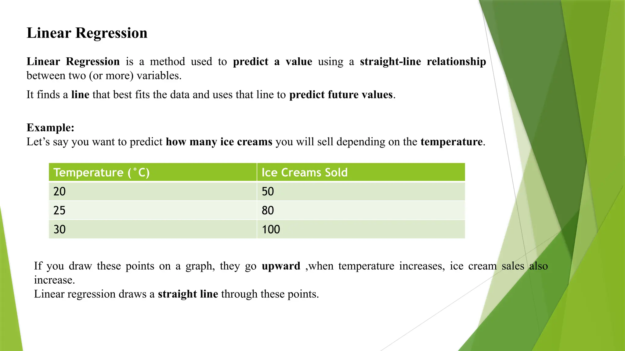
Linear Regression Linear Regression is a method used to predict a value using a straight-line relationship between two (or more) variables. It finds a line that best fits the data and uses that line to predict future values. Example: Let’s say you want to predict how many ice creams you will sell depending on the temperature. Temperature (°C) Ice Creams Sold 20 50 25 80 30 100 If you draw these points on a graph, they go upward ,when temperature increases, ice cream sales also increase. Linear regression draws a straight line through these points.

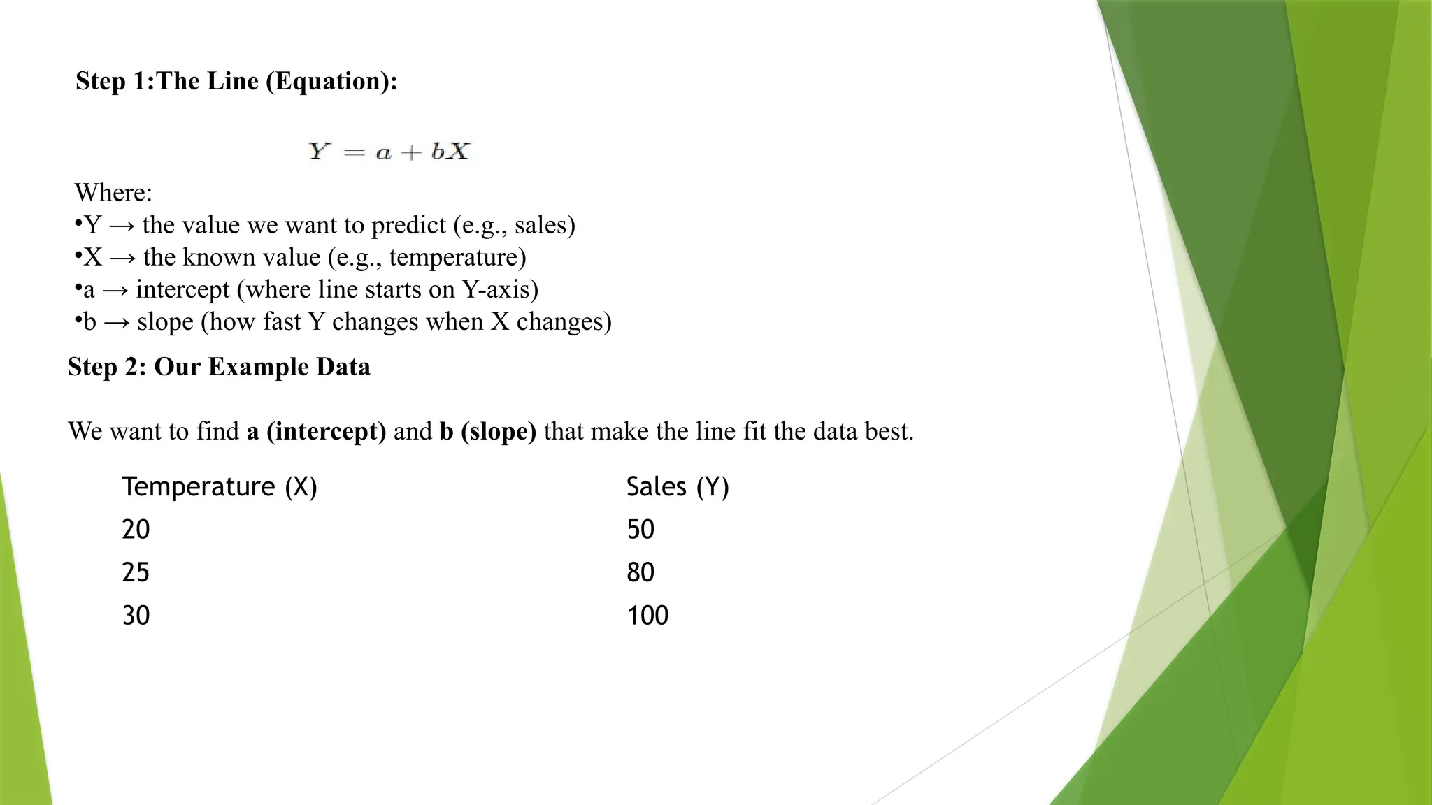
Step 1:The Line (Equation): Where: •Y → the value we want to predict (e.g., sales) •X → the known value (e.g., temperature) •a → intercept (where line starts on Y-axis) •b → slope (how fast Y changes when X changes) Temperature (X) Sales (Y) 20 50 25 80 30 100 Step 2: Our Example Data We want to find a (intercept) and b (slope) that make the line fit the data best.

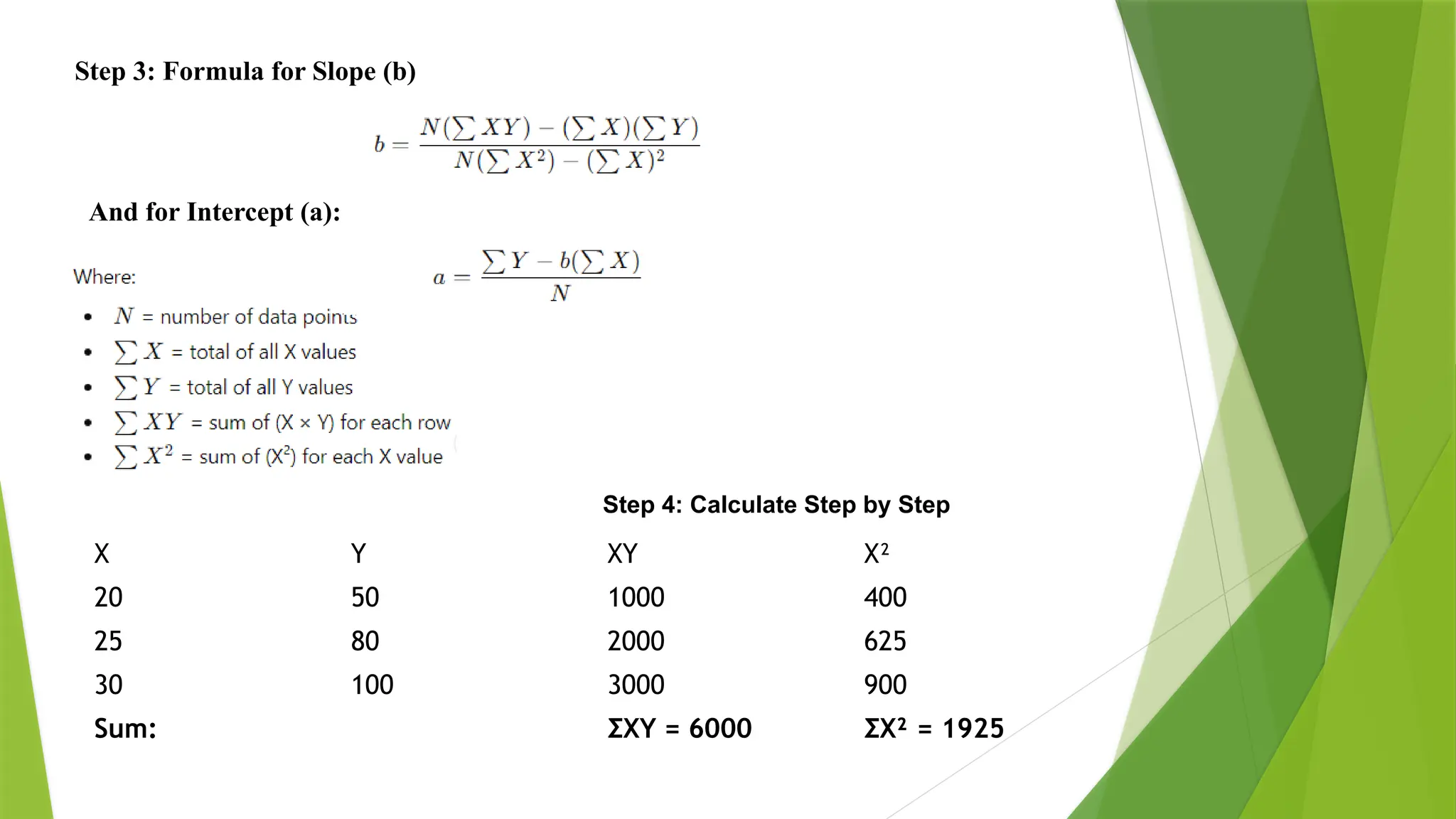
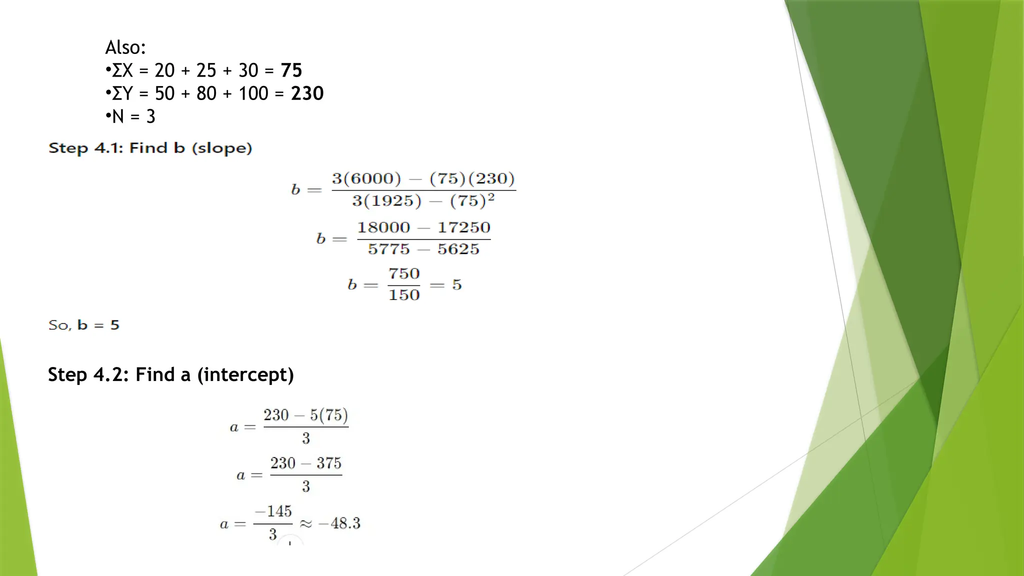
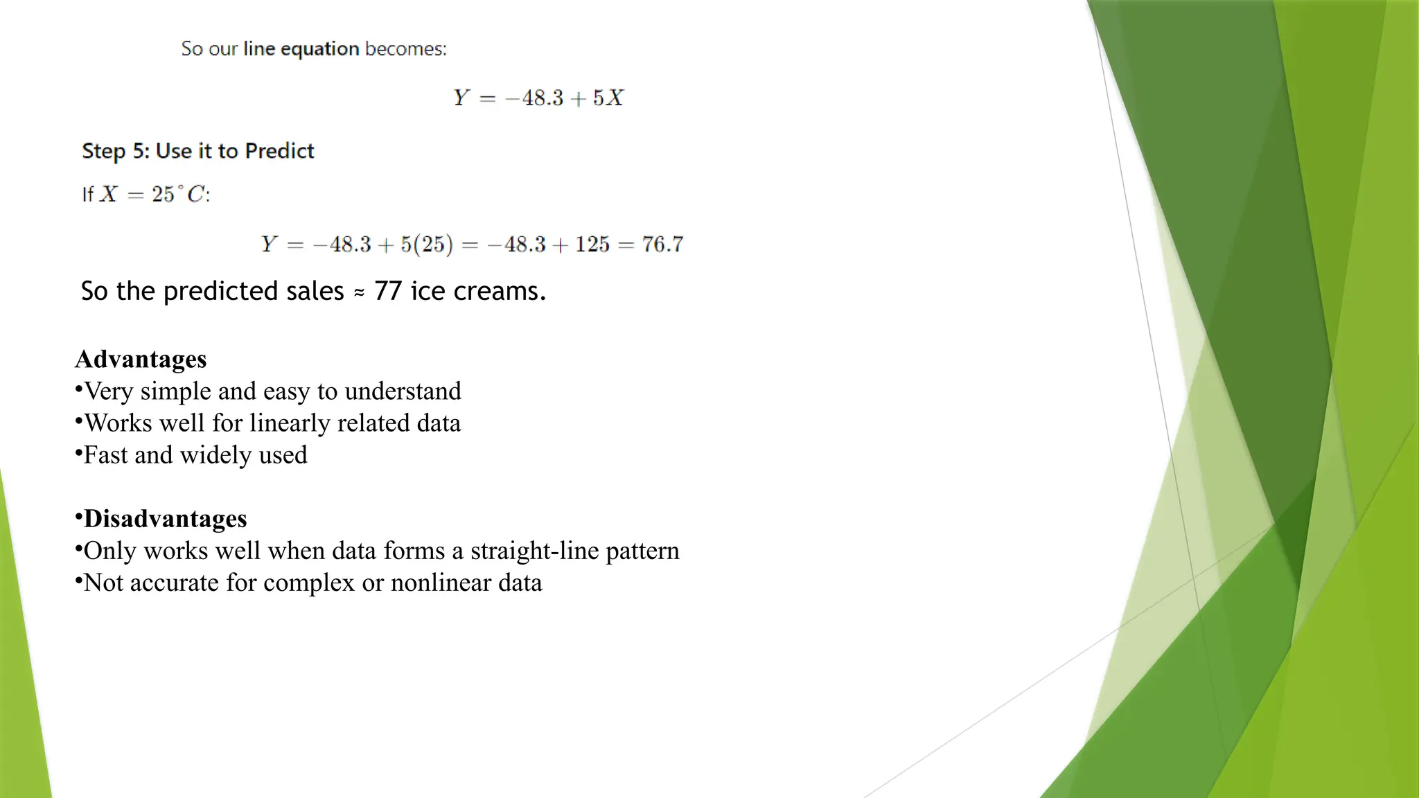
Step 3: Formula for Slope (b) And for Intercept (a): X Y XY X² 20 50 1000 400 25 80 2000 625 30 100 3000 900 Sum: ΣXY = 6000 ΣX² = 1925 Step 4: Calculate Step by Step

Also: •ΣX = 20 + 25 + 30 = 75 •ΣY = 50 + 80 + 100 = 230 •N = 3 Step 4.2: Find a (intercept)

So the predicted sales ≈ 77 ice creams. Advantages •Very simple and easy to understand •Works well for linearly related data •Fast and widely used •Disadvantages •Only works well when data forms a straight-line pattern •Not accurate for complex or nonlinear data

CLASSIFICATION METHODS IN DATA MINING AND MODELING

More Related Content

Similar to CLASSIFICATION METHODS IN DATA MINING AND MODELING

Recently uploaded

CLASSIFICATION METHODS IN DATA MINING AND MODELING