U.V Vandebona
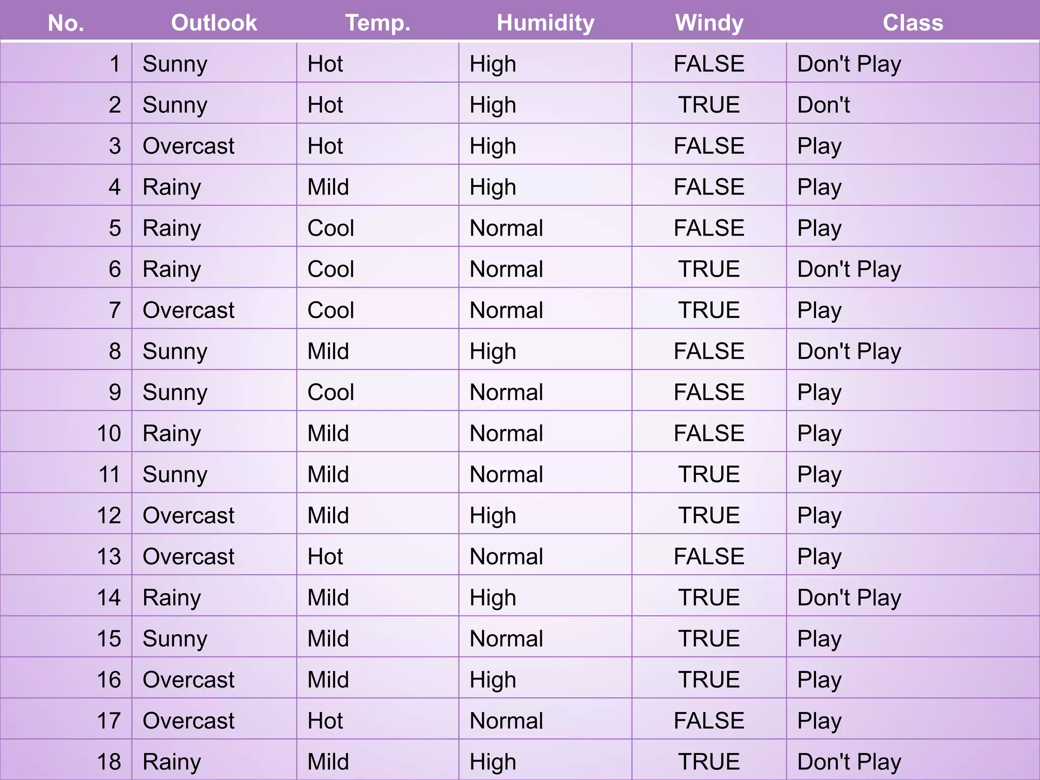
No. Outlook Temp. Humidity Windy Class 1 Sunny Hot High FALSE Don't Play 2 Sunny Hot High TRUE Don't 3 Overcast Hot High FALSE Play 4 Rainy Mild High FALSE Play 5 Rainy Cool Normal FALSE Play 6 Rainy Cool Normal TRUE Don't Play 7 Overcast Cool Normal TRUE Play 8 Sunny Mild High FALSE Don't Play 9 Sunny Cool Normal FALSE Play 10 Rainy Mild Normal FALSE Play 11 Sunny Mild Normal TRUE Play 12 Overcast Mild High TRUE Play 13 Overcast Hot Normal FALSE Play 14 Rainy Mild High TRUE Don't Play 15 Sunny Mild Normal TRUE Play 16 Overcast Mild High TRUE Play 17 Overcast Hot Normal FALSE Play 18 Rainy Mild High TRUE Don't Play
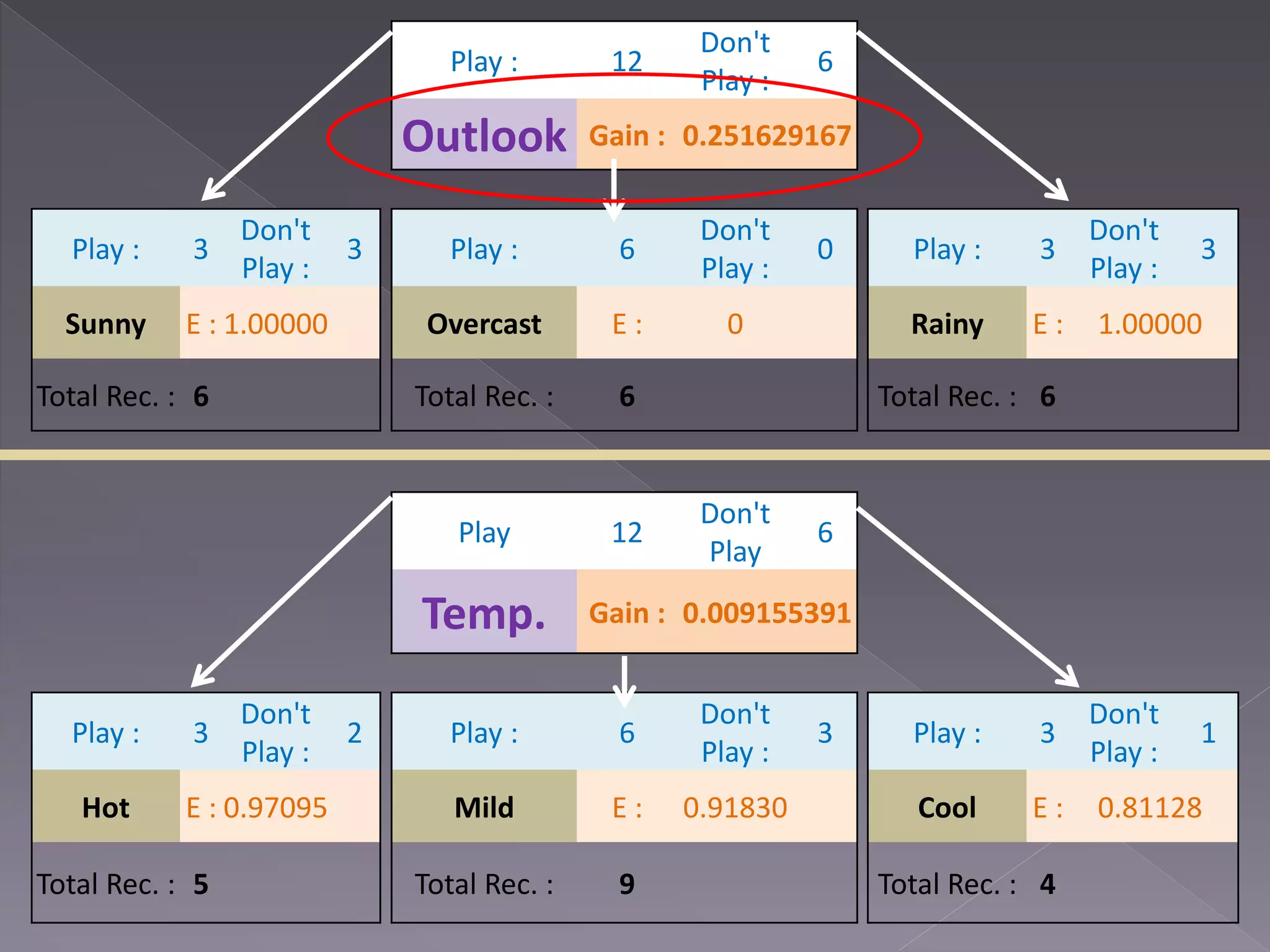
Play : 12 Don't Play : 6 Outlook Gain : 0.251629167 Play : 3 Don't Play : 3 Play : 6 Don't Play : 0 Play : 3 Don't Play : 3 Sunny E : 1.00000 Overcast E : 0 Rainy E : 1.00000 Total Rec. : 6 Total Rec. : 6 Total Rec. : 6 Play 12 Don't Play 6 Temp. Gain : 0.009155391 Play : 3 Don't Play : 2 Play : 6 Don't Play : 3 Play : 3 Don't Play : 1 Hot E : 0.97095 Mild E : 0.91830 Cool E : 0.81128 Total Rec. : 5 Total Rec. : 9 Total Rec. : 4
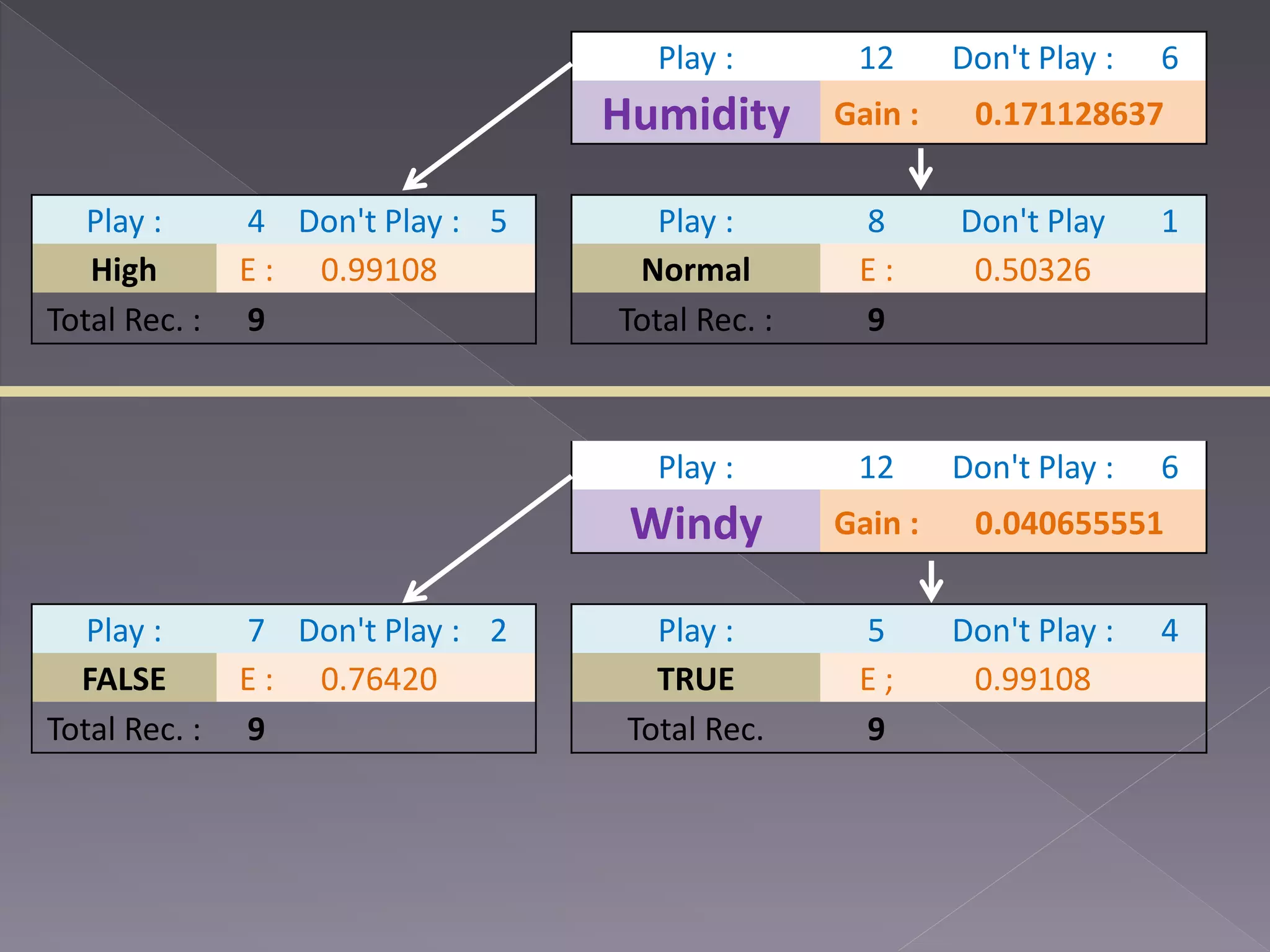
Play : 12 Don't Play : 6 Humidity Gain : 0.171128637 Play : 4 Don't Play : 5 Play : 8 Don't Play 1 High E : 0.99108 Normal E : 0.50326 Total Rec. : 9 Total Rec. : 9 Play : 12 Don't Play : 6 Windy Gain : 0.040655551 Play : 7 Don't Play : 2 Play : 5 Don't Play : 4 FALSE E : 0.76420 TRUE E ; 0.99108 Total Rec. : 9 Total Rec. 9
Outlook Sunny ? Overcast [Play] Rain ?
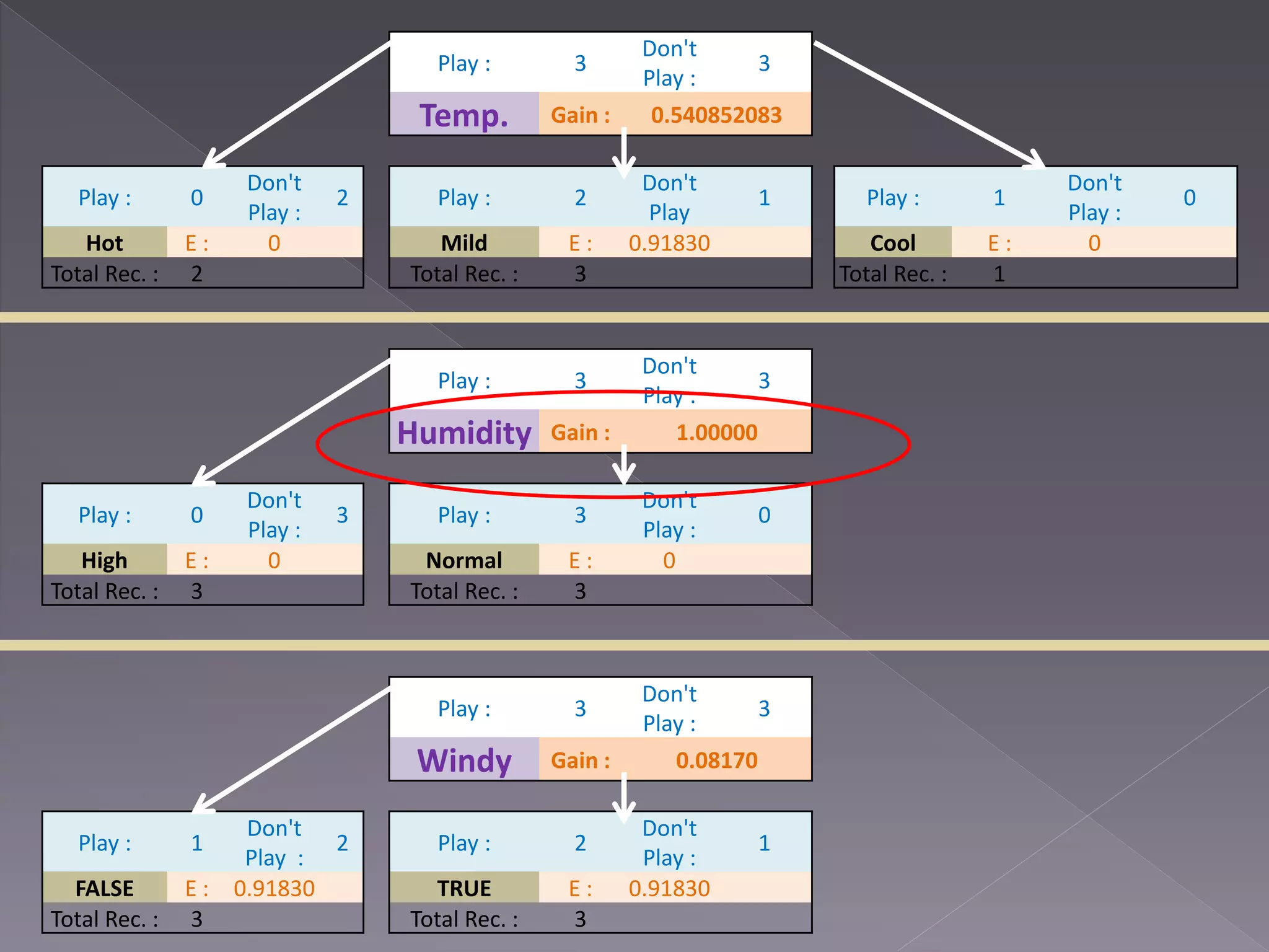
Play : 3 Don't Play : 3 Temp. Gain : 0.540852083 Play : 0 Don't Play : 2 Play : 2 Don't Play 1 Play : 1 Don't Play : 0 Hot E : 0 Mild E : 0.91830 Cool E : 0 Total Rec. : 2 Total Rec. : 3 Total Rec. : 1 Play : 3 Don't Play : 3 Humidity Gain : 1.00000 Play : 0 Don't Play : 3 Play : 3 Don't Play : 0 High E : 0 Normal E : 0 Total Rec. : 3 Total Rec. : 3 Play : 3 Don't Play : 3 Windy Gain : 0.08170 Play : 1 Don't Play : 2 Play : 2 Don't Play : 1 FALSE E : 0.91830 TRUE E : 0.91830 Total Rec. : 3 Total Rec. : 3
Outlook Sunny Humidity High [Don’t Play] Normal [Play] Overcast [Play] Rain ?
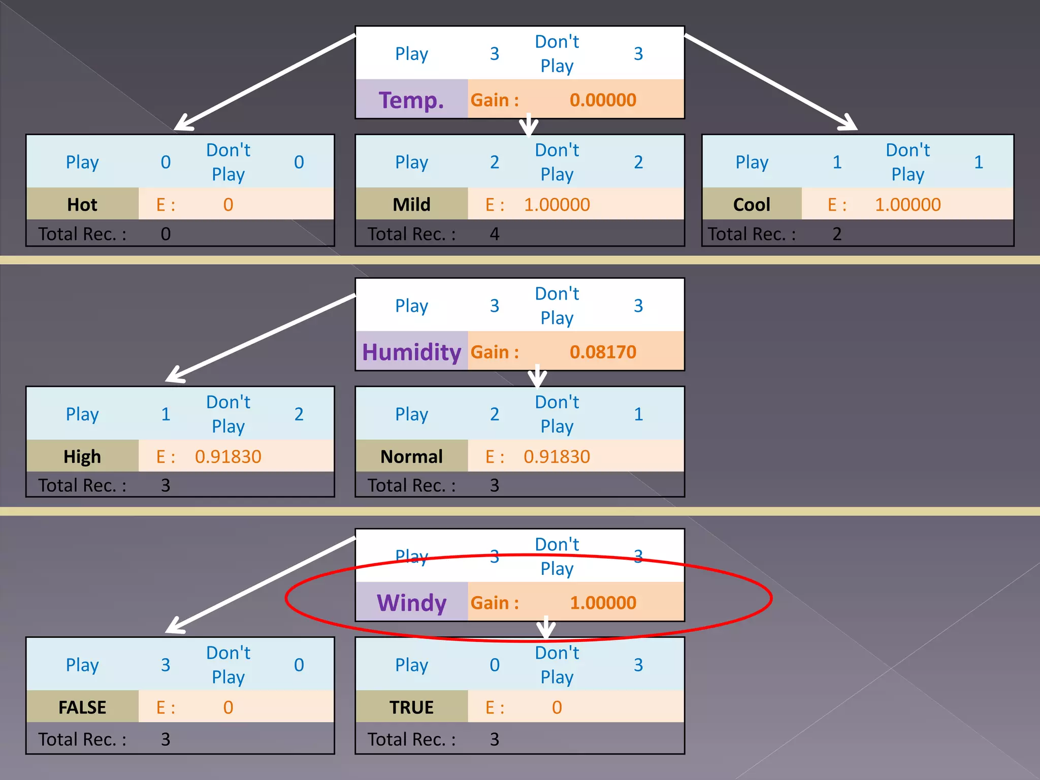
Play 3 Don't Play 3 Temp. Gain : 0.00000 Play 0 Don't Play 0 Play 2 Don't Play 2 Play 1 Don't Play 1 Hot E : 0 Mild E : 1.00000 Cool E : 1.00000 Total Rec. : 0 Total Rec. : 4 Total Rec. : 2 Play 3 Don't Play 3 Humidity Gain : 0.08170 Play 1 Don't Play 2 Play 2 Don't Play 1 High E : 0.91830 Normal E : 0.91830 Total Rec. : 3 Total Rec. : 3 Play 3 Don't Play 3 Windy Gain : 1.00000 Play 3 Don't Play 0 Play 0 Don't Play 3 FALSE E : 0 TRUE E : 0 Total Rec. : 3 Total Rec. : 3
Outlook Sunny Humidity High [Don’t Play] Normal [Play] Overcast [Play] Rain Windy False [Play] True [Don’t Play] Final Decision Tree
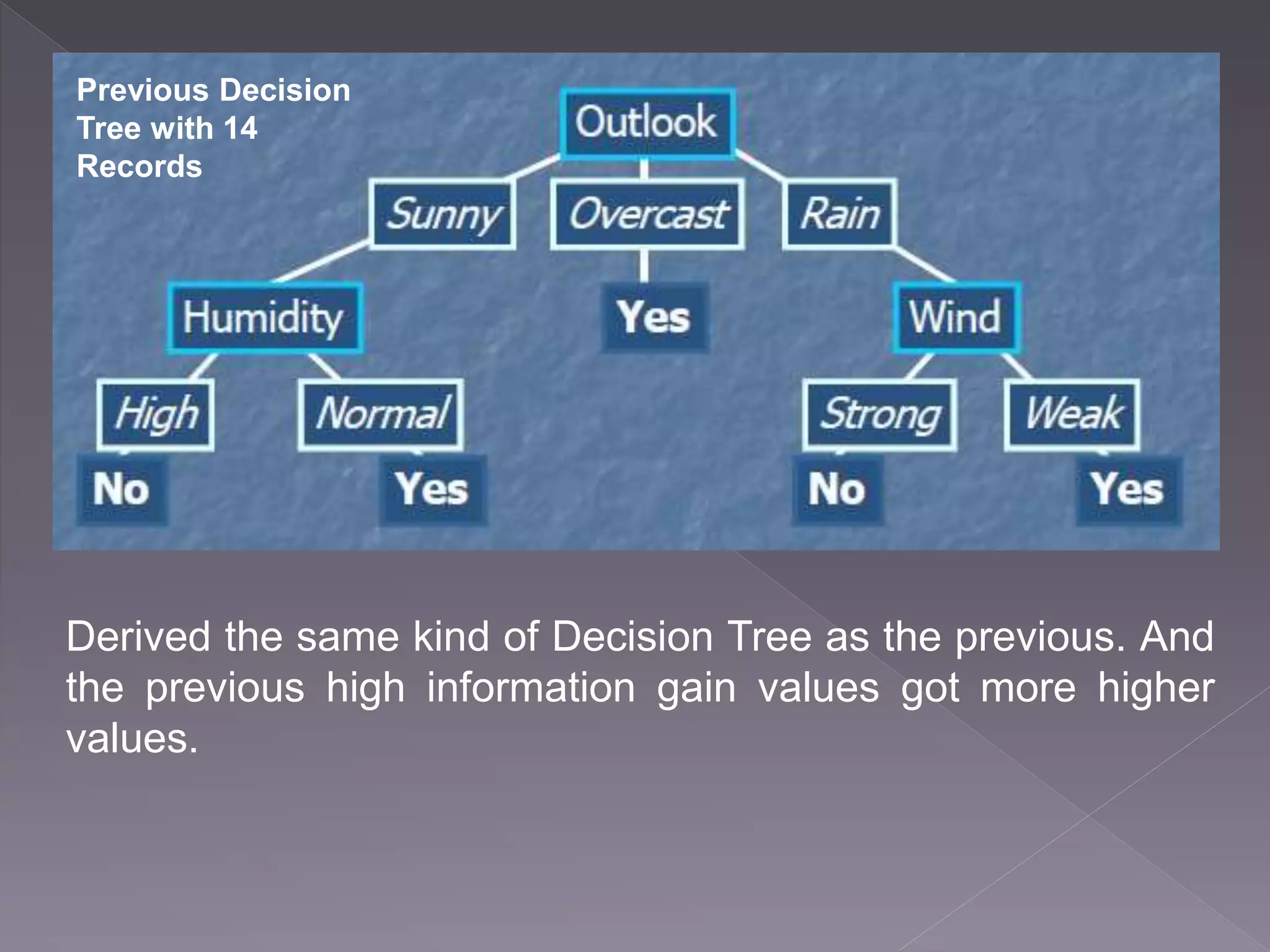
Previous Decision Tree with 14 Records Derived the same kind of Decision Tree as the previous. And the previous high information gain values got more higher values.
U.V Vandebona (MCS/2013/072) Index No : 13440722
 Twitter analysis aims to detect the class the tweet is belongs to.  For example if classes are positive & negative: › “Have a nice day!”  Algorithm should tell that this is a positive message. › “I had a bad day”  Algorithm should tell that this is a negative message.
 From the machine learning domain point of view this can be seen as a classification task and naive Bayes is an algorithm which suits well for this kind of a task.  The naive Bayes algorithm uses probabilities to decide which class best matches for a given input text.
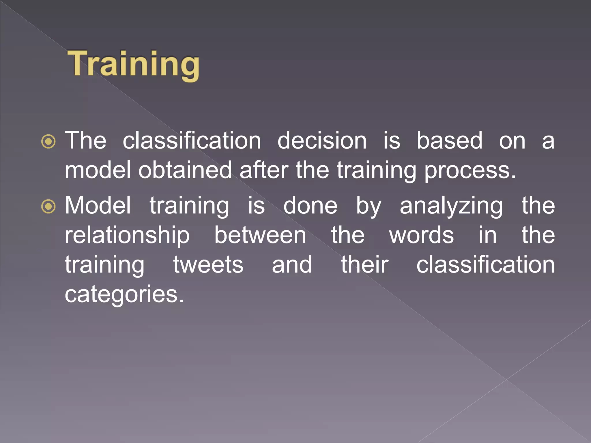
 The classification decision is based on a model obtained after the training process.  Model training is done by analyzing the relationship between the words in the training tweets and their classification categories.
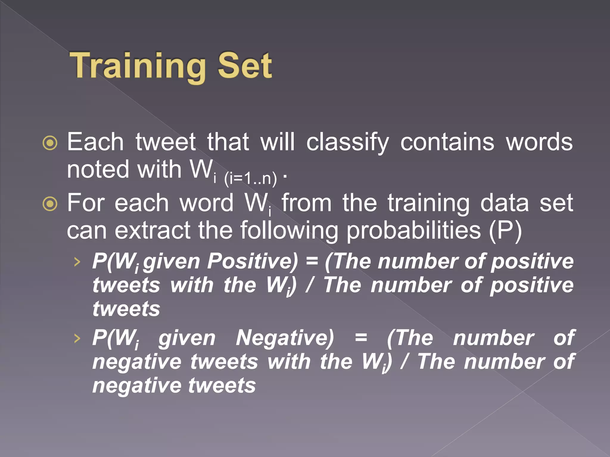
 Each tweet that will classify contains words noted with Wi (i=1..n) .  For each word Wi from the training data set can extract the following probabilities (P) › P(Wi given Positive) = (The number of positive tweets with the Wi) / The number of positive tweets › P(Wi given Negative) = (The number of negative tweets with the Wi) / The number of negative tweets
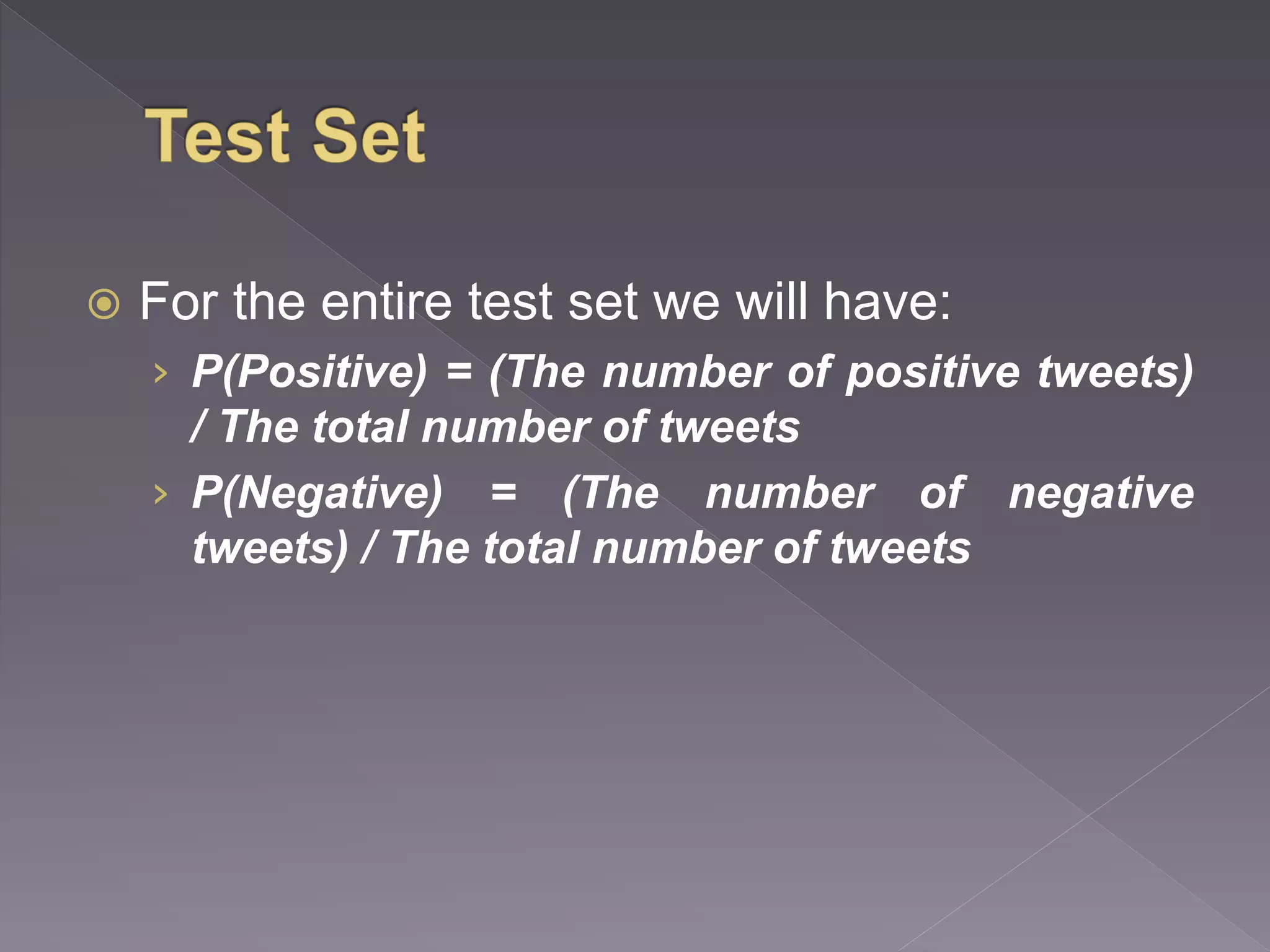
 For the entire test set we will have: › P(Positive) = (The number of positive tweets) / The total number of tweets › P(Negative) = (The number of negative tweets) / The total number of tweets
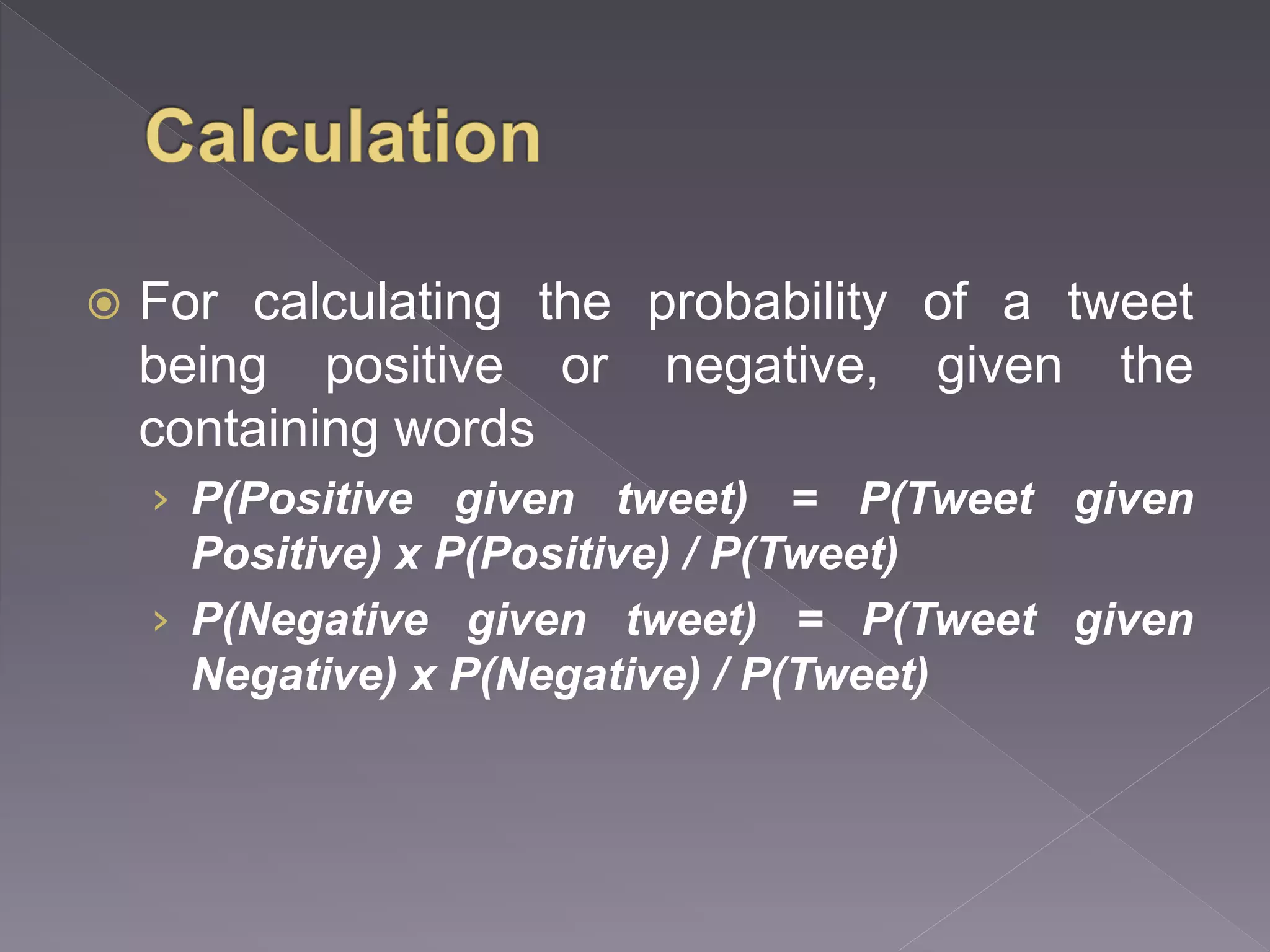
 For calculating the probability of a tweet being positive or negative, given the containing words › P(Positive given tweet) = P(Tweet given Positive) x P(Positive) / P(Tweet) › P(Negative given tweet) = P(Tweet given Negative) x P(Negative) / P(Tweet)
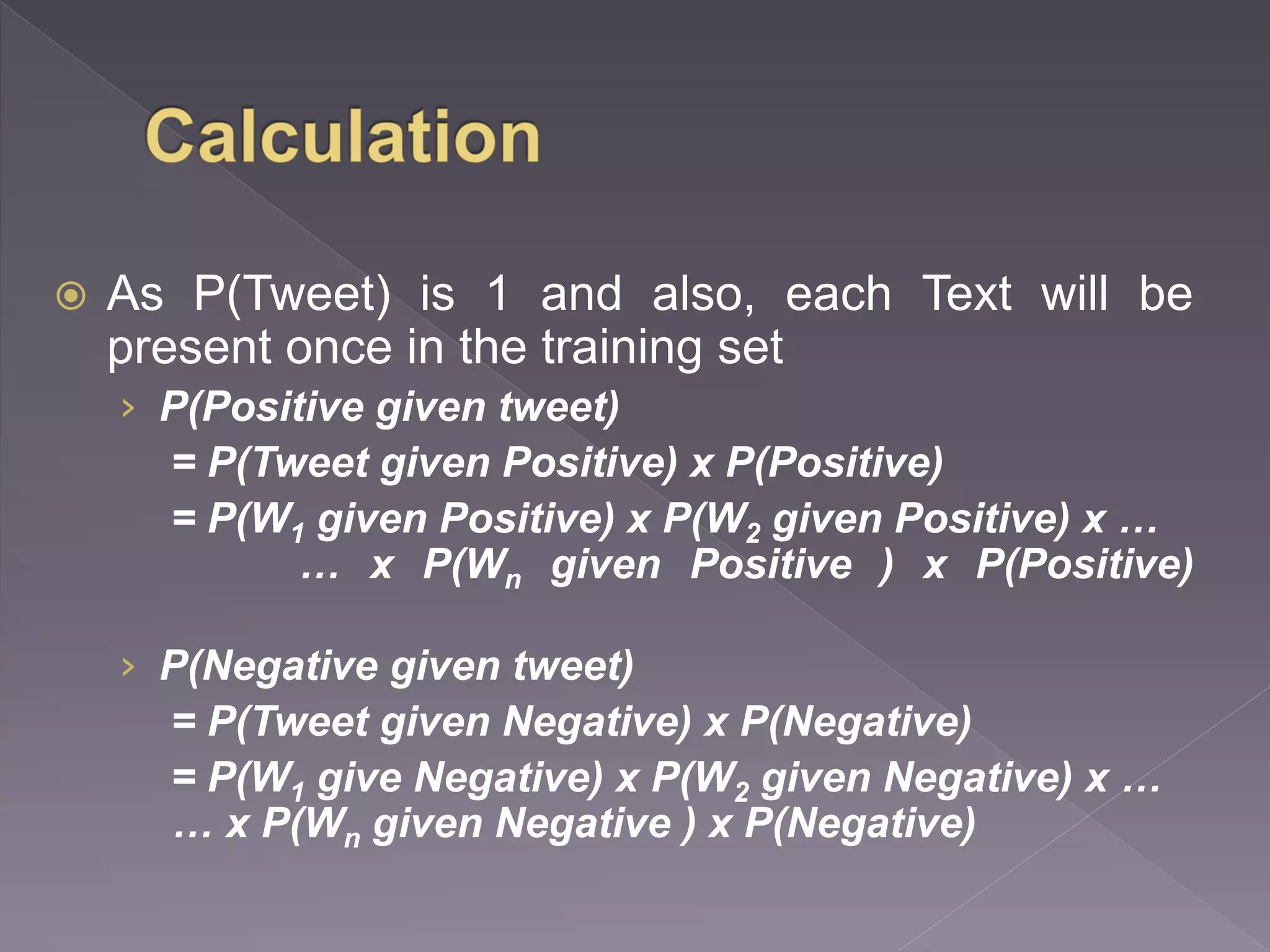
 As P(Tweet) is 1 and also, each Text will be present once in the training set › P(Positive given tweet) = P(Tweet given Positive) x P(Positive) = P(W1 given Positive) x P(W2 given Positive) x … … x P(Wn given Positive ) x P(Positive) › P(Negative given tweet) = P(Tweet given Negative) x P(Negative) = P(W1 give Negative) x P(W2 given Negative) x … … x P(Wn given Negative ) x P(Negative)
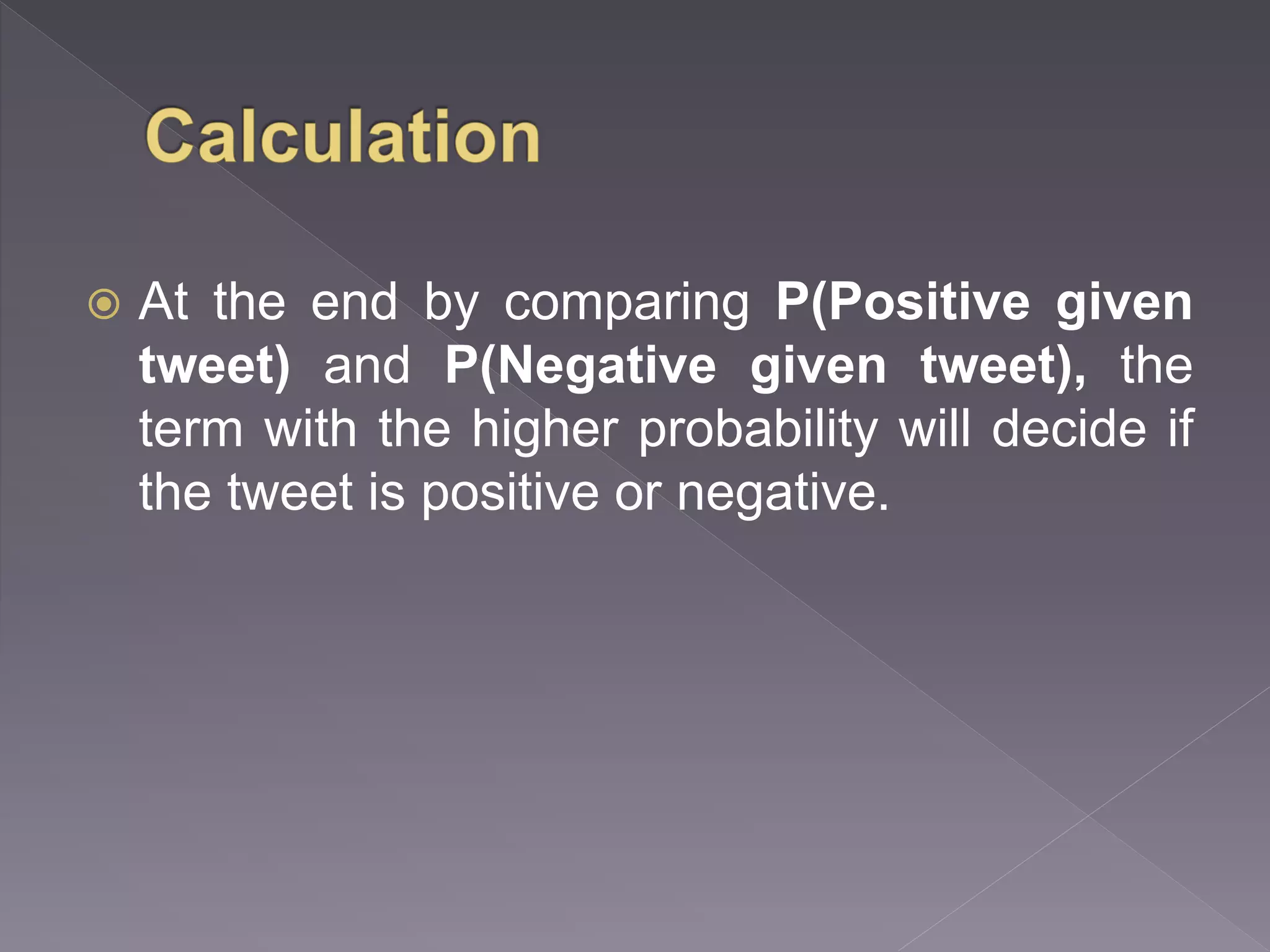
 At the end by comparing P(Positive given tweet) and P(Negative given tweet), the term with the higher probability will decide if the tweet is positive or negative.
 http://technobium.com/sentiment- analysis-using-mahout-naive-bayes/ [Online - 2015/11/11]

Data Analytics and Machine Learning

  • 1.
  • 2.
    No. Outlook Temp.Humidity Windy Class 1 Sunny Hot High FALSE Don't Play 2 Sunny Hot High TRUE Don't 3 Overcast Hot High FALSE Play 4 Rainy Mild High FALSE Play 5 Rainy Cool Normal FALSE Play 6 Rainy Cool Normal TRUE Don't Play 7 Overcast Cool Normal TRUE Play 8 Sunny Mild High FALSE Don't Play 9 Sunny Cool Normal FALSE Play 10 Rainy Mild Normal FALSE Play 11 Sunny Mild Normal TRUE Play 12 Overcast Mild High TRUE Play 13 Overcast Hot Normal FALSE Play 14 Rainy Mild High TRUE Don't Play 15 Sunny Mild Normal TRUE Play 16 Overcast Mild High TRUE Play 17 Overcast Hot Normal FALSE Play 18 Rainy Mild High TRUE Don't Play
  • 3.
    Play : 12 Don't Play: 6 Outlook Gain : 0.251629167 Play : 3 Don't Play : 3 Play : 6 Don't Play : 0 Play : 3 Don't Play : 3 Sunny E : 1.00000 Overcast E : 0 Rainy E : 1.00000 Total Rec. : 6 Total Rec. : 6 Total Rec. : 6 Play 12 Don't Play 6 Temp. Gain : 0.009155391 Play : 3 Don't Play : 2 Play : 6 Don't Play : 3 Play : 3 Don't Play : 1 Hot E : 0.97095 Mild E : 0.91830 Cool E : 0.81128 Total Rec. : 5 Total Rec. : 9 Total Rec. : 4
  • 4.
    Play : 12Don't Play : 6 Humidity Gain : 0.171128637 Play : 4 Don't Play : 5 Play : 8 Don't Play 1 High E : 0.99108 Normal E : 0.50326 Total Rec. : 9 Total Rec. : 9 Play : 12 Don't Play : 6 Windy Gain : 0.040655551 Play : 7 Don't Play : 2 Play : 5 Don't Play : 4 FALSE E : 0.76420 TRUE E ; 0.99108 Total Rec. : 9 Total Rec. 9
  • 5.
  • 6.
    Play : 3 Don't Play: 3 Temp. Gain : 0.540852083 Play : 0 Don't Play : 2 Play : 2 Don't Play 1 Play : 1 Don't Play : 0 Hot E : 0 Mild E : 0.91830 Cool E : 0 Total Rec. : 2 Total Rec. : 3 Total Rec. : 1 Play : 3 Don't Play : 3 Humidity Gain : 1.00000 Play : 0 Don't Play : 3 Play : 3 Don't Play : 0 High E : 0 Normal E : 0 Total Rec. : 3 Total Rec. : 3 Play : 3 Don't Play : 3 Windy Gain : 0.08170 Play : 1 Don't Play : 2 Play : 2 Don't Play : 1 FALSE E : 0.91830 TRUE E : 0.91830 Total Rec. : 3 Total Rec. : 3
  • 7.
  • 8.
    Play 3 Don't Play 3 Temp. Gain: 0.00000 Play 0 Don't Play 0 Play 2 Don't Play 2 Play 1 Don't Play 1 Hot E : 0 Mild E : 1.00000 Cool E : 1.00000 Total Rec. : 0 Total Rec. : 4 Total Rec. : 2 Play 3 Don't Play 3 Humidity Gain : 0.08170 Play 1 Don't Play 2 Play 2 Don't Play 1 High E : 0.91830 Normal E : 0.91830 Total Rec. : 3 Total Rec. : 3 Play 3 Don't Play 3 Windy Gain : 1.00000 Play 3 Don't Play 0 Play 0 Don't Play 3 FALSE E : 0 TRUE E : 0 Total Rec. : 3 Total Rec. : 3
  • 9.
  • 10.
    Previous Decision Tree with14 Records Derived the same kind of Decision Tree as the previous. And the previous high information gain values got more higher values.
  • 11.
  • 12.
     Twitter analysisaims to detect the class the tweet is belongs to.  For example if classes are positive & negative: › “Have a nice day!”  Algorithm should tell that this is a positive message. › “I had a bad day”  Algorithm should tell that this is a negative message.
  • 13.
     From themachine learning domain point of view this can be seen as a classification task and naive Bayes is an algorithm which suits well for this kind of a task.  The naive Bayes algorithm uses probabilities to decide which class best matches for a given input text.
  • 14.
     The classificationdecision is based on a model obtained after the training process.  Model training is done by analyzing the relationship between the words in the training tweets and their classification categories.
  • 15.
     Each tweetthat will classify contains words noted with Wi (i=1..n) .  For each word Wi from the training data set can extract the following probabilities (P) › P(Wi given Positive) = (The number of positive tweets with the Wi) / The number of positive tweets › P(Wi given Negative) = (The number of negative tweets with the Wi) / The number of negative tweets
  • 16.
     For theentire test set we will have: › P(Positive) = (The number of positive tweets) / The total number of tweets › P(Negative) = (The number of negative tweets) / The total number of tweets
  • 17.
     For calculatingthe probability of a tweet being positive or negative, given the containing words › P(Positive given tweet) = P(Tweet given Positive) x P(Positive) / P(Tweet) › P(Negative given tweet) = P(Tweet given Negative) x P(Negative) / P(Tweet)
  • 18.
     As P(Tweet)is 1 and also, each Text will be present once in the training set › P(Positive given tweet) = P(Tweet given Positive) x P(Positive) = P(W1 given Positive) x P(W2 given Positive) x … … x P(Wn given Positive ) x P(Positive) › P(Negative given tweet) = P(Tweet given Negative) x P(Negative) = P(W1 give Negative) x P(W2 given Negative) x … … x P(Wn given Negative ) x P(Negative)
  • 19.
     At theend by comparing P(Positive given tweet) and P(Negative given tweet), the term with the higher probability will decide if the tweet is positive or negative.
  • 20.

Editor's Notes

  • #14 The algorithm is considered naive because it assumes that the value of a particular feature is independent of the value of any other feature, given the class variable. For example, a fruit may be considered to be an apple if it is red, round, and about 3″ in diameter. A naive Bayes classifier considers each of these features to contribute independently to the probability that this fruit is an apple, regardless of any possible correlations between the color, roundness and diameter features