DBMS Query Optimization along with algorithms

Chapter 15 (TCDS) Sukarna Barua Associate Professor, CSE, BUET 6/27/2025

The Query Processor  Functions of query processor:  Converts high level SQL queries into a sequence of database operations and executes those operations.  Converts high level query to a detailed description.  Use query algorithms to efficiently execute a query. 6/27/2025

The Query Processor  Major approaches in query processing:  Scanning, hashing, sorting, and indexing  Algorithms have significantly different costs and structures:  Some algorithms assume main memory is available at least one of the relations involved in an operation.  Others assume that the arguments are too big to fit in the main memory.  Query processing has two parts:  Query compilation  Query execution. 6/27/2025

Query Compilation  Three major steps in query compilation: (a) Parsing:  Checks the syntax and semantics of the query.  A parse tree (or syntax tree) is constructed from the SQL query.  Also known as expression tree. [ when parse tree is represented using relational algebra operators]  This representation is more succinct.  Example: Parse tree shown (right) for the given SQL (left). 6/27/2025

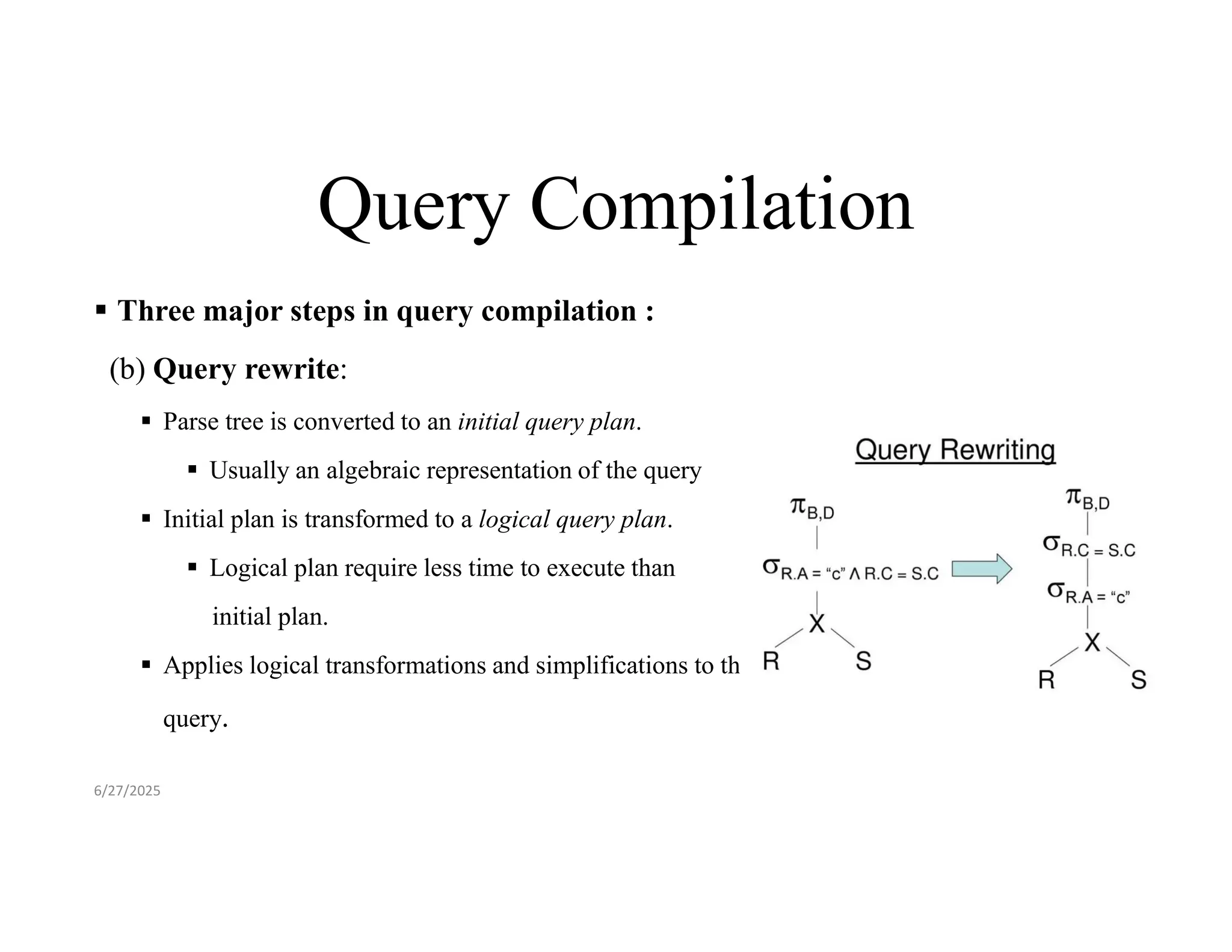
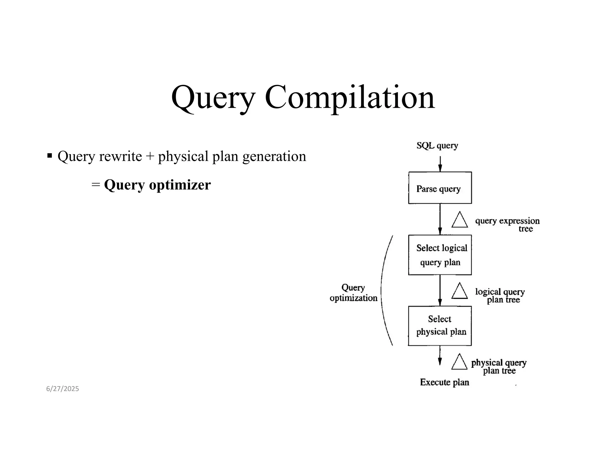
Query Compilation  Three major steps in query compilation : (b) Query rewrite:  Parse tree is converted to an initial query plan.  Usually an algebraic representation of the query  Initial plan is transformed to a logical query plan.  Logical plan require less time to execute than initial plan.  Applies logical transformations and simplifications to the query. 6/27/2025

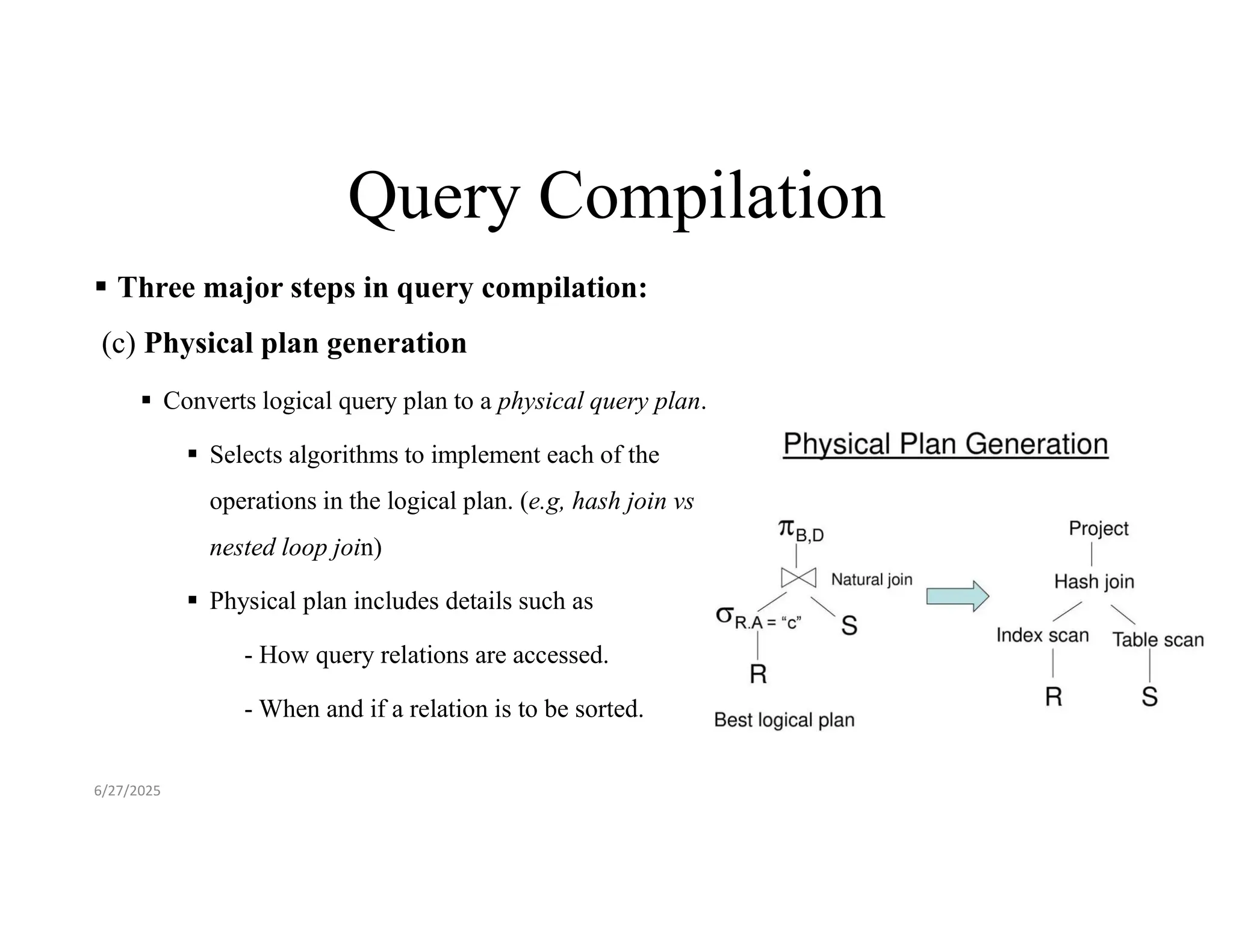
Query Compilation  Three major steps in query compilation: (c) Physical plan generation  Converts logical query plan to a physical query plan.  Selects algorithms to implement each of the operations in the logical plan. (e.g, hash join vs nested loop join)  Physical plan includes details such as - How query relations are accessed. - When and if a relation is to be sorted. 6/27/2025

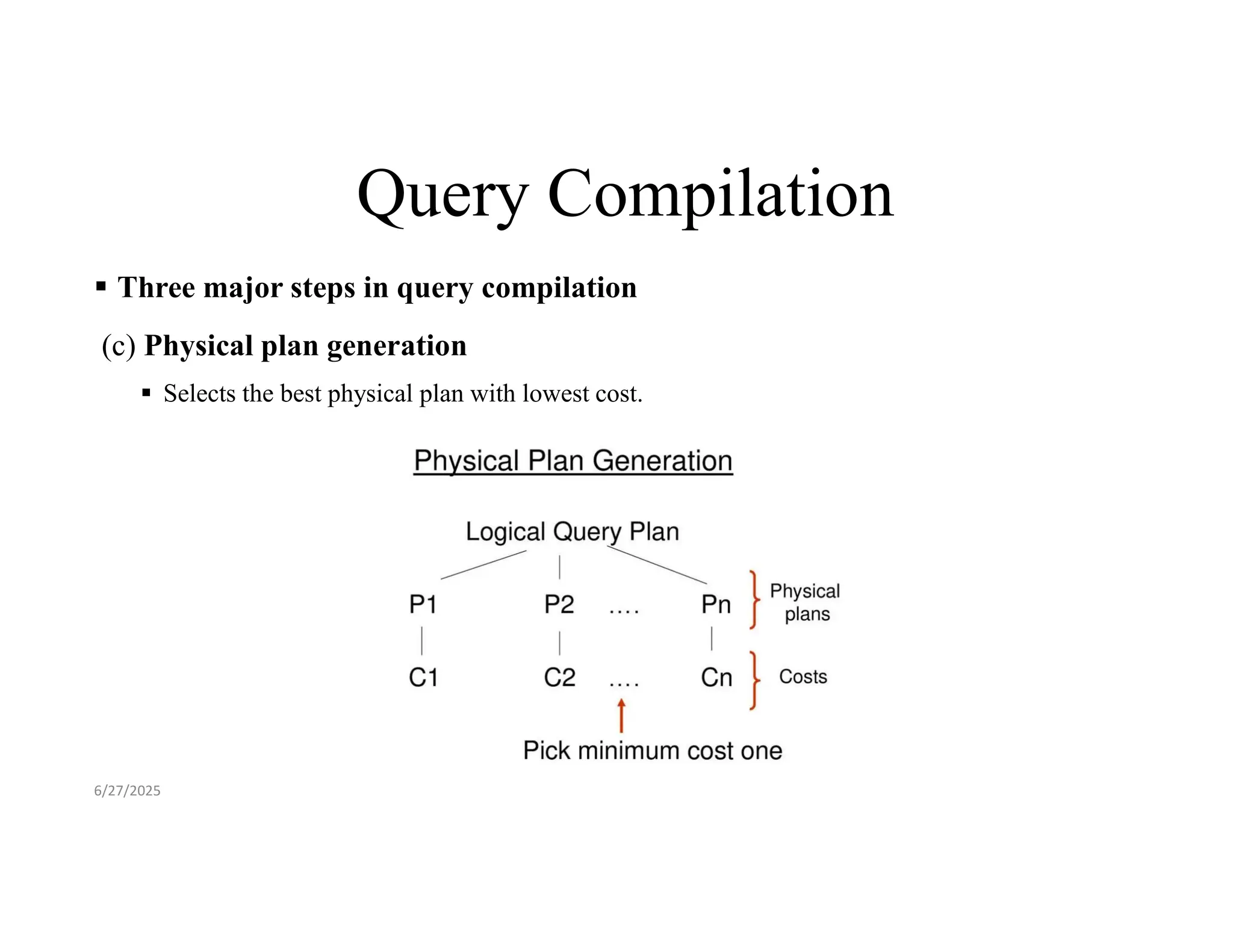
Query Compilation  Three major steps in query compilation (c) Physical plan generation  Selects the best physical plan with lowest cost. 6/27/2025

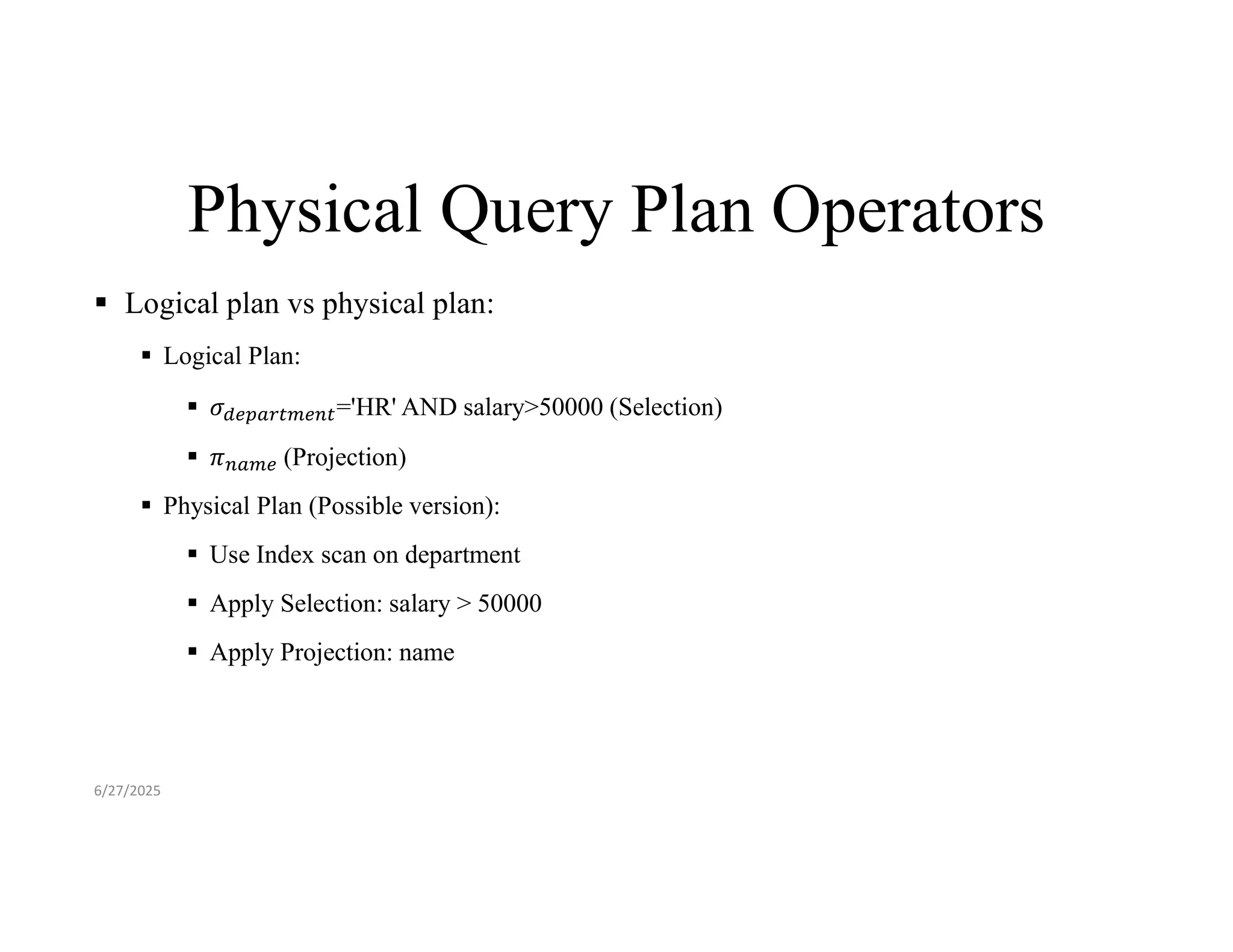
Physical Query Plan Operators  Logical plan vs physical plan:  Logical Plan:  𝜎 ='HR' AND salary>50000 (Selection)  𝜋 (Projection)  Physical Plan (Possible version):  Use Index scan on department  Apply Selection: salary > 50000  Apply Projection: name 6/27/2025

Query Compilation  Query rewrite + physical plan generation = Query optimizer 6/27/2025

Issues to Consider  Issue 1: What is the algebraically equivalent forms of a query that leads to the most efficient algorithms for answering the query?  Issue 2: For each operation, what algorithms should be used to implement that operation?  Issue 3: How should the operations pass data from one to the other, e.g., in a pipelined fashion, in memory buffers, or via the disk? 6/27/2025

Metadata for Best Query Plan Generation  Metadata to consider for best query plan generation:  1 - The size of each relation  The number of rows (tuples) in each table (relation).  Helps estimate how long it will take to scan a table or join it with another.  A small table can be scanned quickly, while a large one might require a more efficient strategy (e.g., using an index or join reordering). 6/27/2025

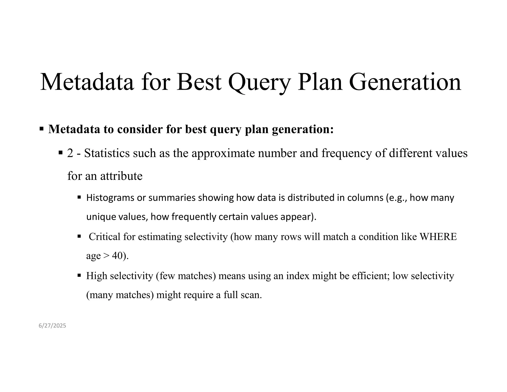
Metadata for Best Query Plan Generation  Metadata to consider for best query plan generation:  2 - Statistics such as the approximate number and frequency of different values for an attribute  Histograms or summaries showing how data is distributed in columns (e.g., how many unique values, how frequently certain values appear).  Critical for estimating selectivity (how many rows will match a condition like WHERE age > 40).  High selectivity (few matches) means using an index might be efficient; low selectivity (many matches) might require a full scan. 6/27/2025

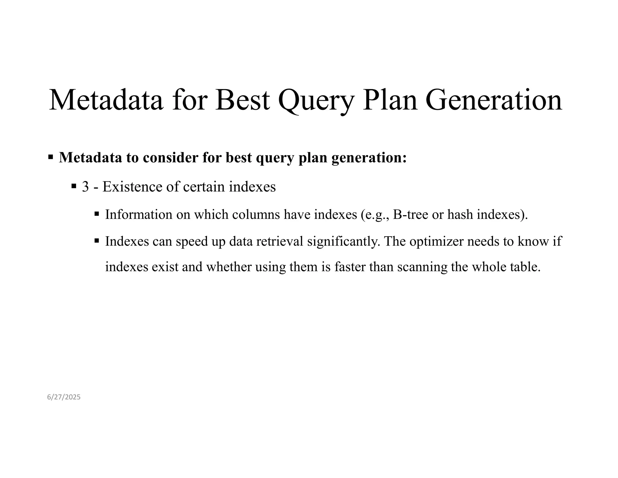
Metadata for Best Query Plan Generation  Metadata to consider for best query plan generation:  3 - Existence of certain indexes  Information on which columns have indexes (e.g., B-tree or hash indexes).  Indexes can speed up data retrieval significantly. The optimizer needs to know if indexes exist and whether using them is faster than scanning the whole table. 6/27/2025

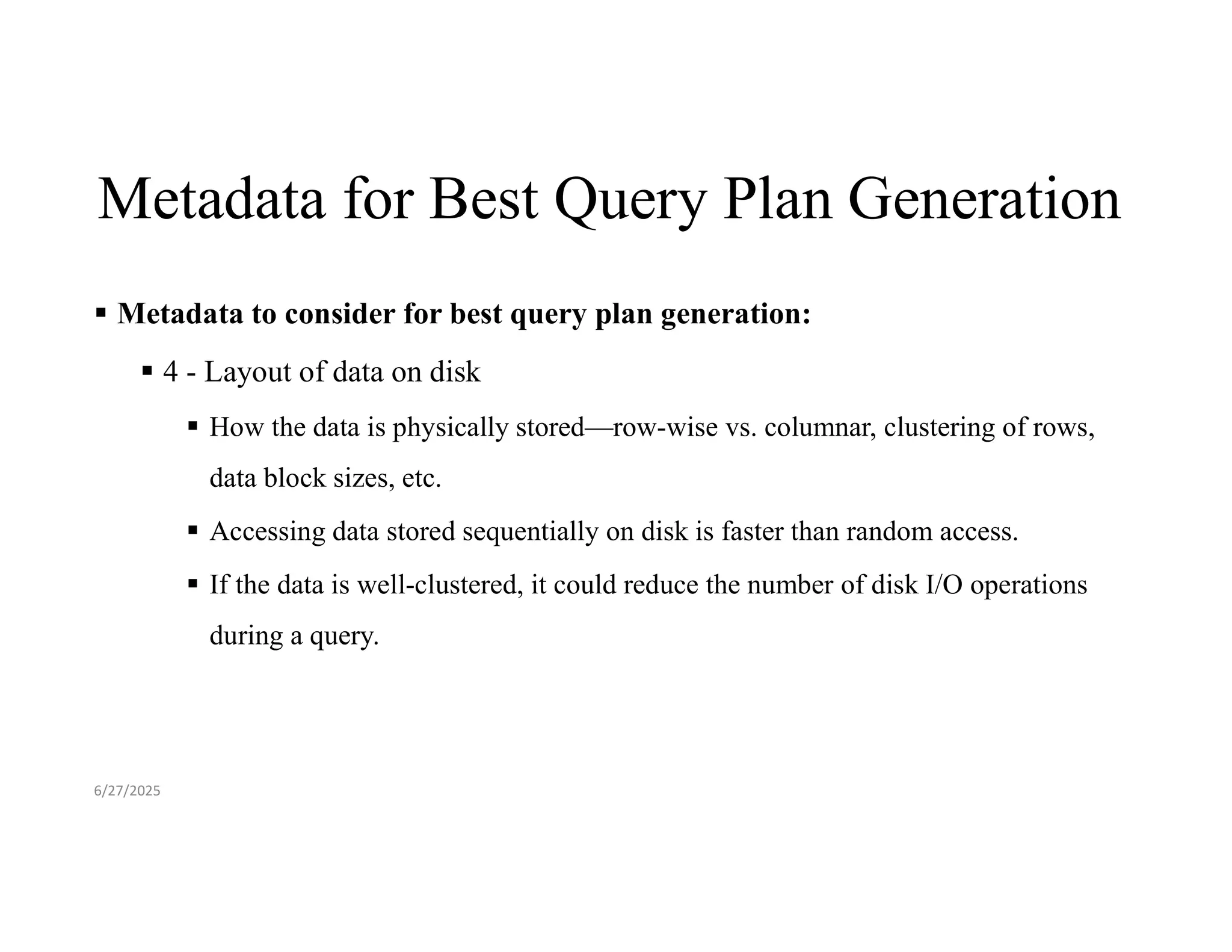
Metadata for Best Query Plan Generation  Metadata to consider for best query plan generation:  4 - Layout of data on disk  How the data is physically stored—row-wise vs. columnar, clustering of rows, data block sizes, etc.  Accessing data stored sequentially on disk is faster than random access.  If the data is well-clustered, it could reduce the number of disk I/O operations during a query. 6/27/2025

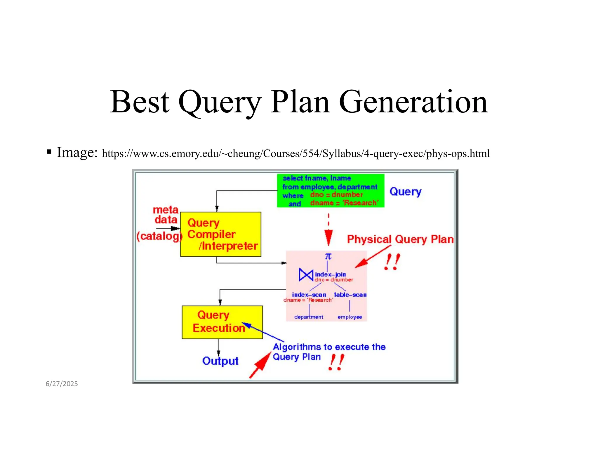
Best Query Plan Generation  Image: https://www.cs.emory.edu/~cheung/Courses/554/Syllabus/4-query-exec/phys-ops.html 6/27/2025

Physical Query Plan Operators  Physical query plans are built from operators  Physical operators implements logical operations  Relational algebra operations:  Selection ( ), projection ( ), join ( ), etc.  Non-relational algebra operation:  Scanning, sorting, hashing, etc.  Table-scan, index-scan, etc. 6/27/2025

Scanning operation  Scanning:  Reads contents of a table (Relation R)  Full table scan:  Read the entire contents of a relation R.  Predicate based scan:  Read only those tuples of R that satisfy a given predicate. 6/27/2025

Indexing • B+ tree index: • Balanced tree structure with multiple levels • Nodes contain ranges of values and pointers to child nodes • Leaf nodes contain the indexed values and pointers to table rows • Efficient for range search. • Preserves order of tuples (when all tuples are retrieved by index). • Hash index: • Array of buckets (hash table) • Uses a hash function to map keys to specific buckets • Each bucket contains pointers to rows with that hash value • Efficient for equality search. • Does not preserve order of tuples (when all tuples are retrieved by index) 6/27/2025

Clustered index • Clustered index: • The rows are stored physically on the disk in sored order of index column’s values. • Usually the leaf nodes of the B+ tree index contains table rows (not pointers to table rows) • Table rows are sorted in the leaf nodes in the order of index column’s values. • No separate storage for the table (index is the table itself) • Only one clustered index per table is allowed (because data rows can only be ordered one way). • Usually built on the primary key. 6/27/2025

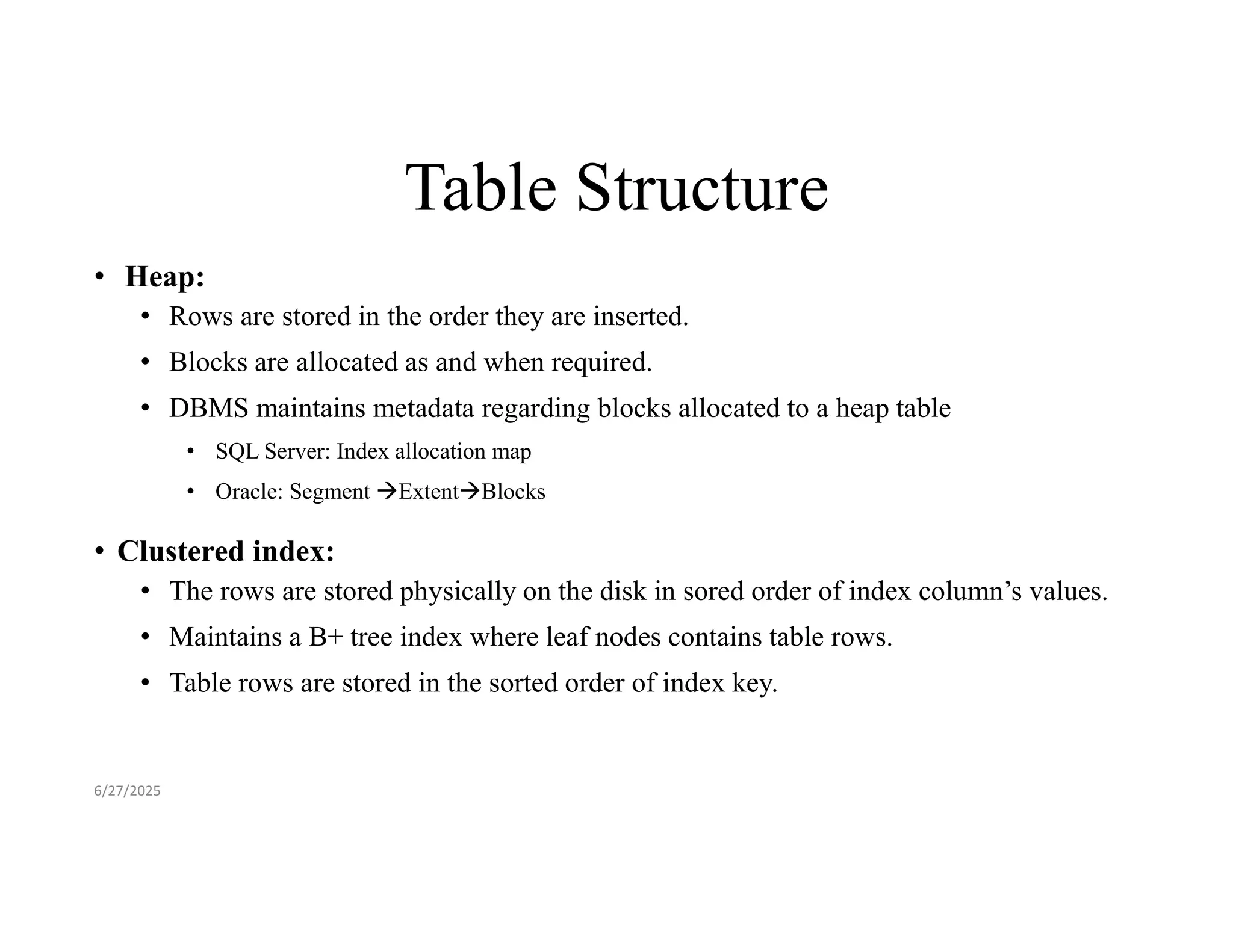
Table Structure • Heap: • Rows are stored in the order they are inserted. • Blocks are allocated as and when required. • DBMS maintains metadata regarding blocks allocated to a heap table • SQL Server: Index allocation map • Oracle: Segment ExtentBlocks • Clustered index: • The rows are stored physically on the disk in sored order of index column’s values. • Maintains a B+ tree index where leaf nodes contains table rows. • Table rows are stored in the sorted order of index key. 6/27/2025

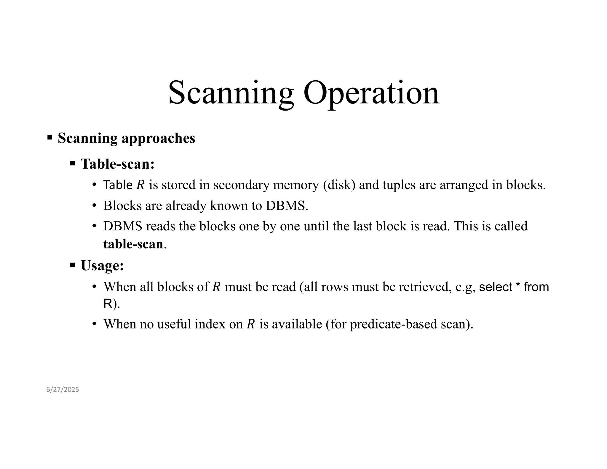
Scanning Operation  Scanning approaches  Table-scan: • Table is stored in secondary memory (disk) and tuples are arranged in blocks. • Blocks are already known to DBMS. • DBMS reads the blocks one by one until the last block is read. This is called table-scan.  Usage: • When all blocks of must be read (all rows must be retrieved, e.g, select * from R). • When no useful index on is available (for predicate-based scan). 6/27/2025

Scanning Operation  Scanning approaches  Index-scan: • An index exists on an attribute of relation • The DBMS reads the index to get the address of blocks and then retrieve the blocks: • The DBMS retrieves all tuples or only those that meet the condition (index seek).  Usage: • When blocks location of are not known to DBMS (all blocks are accessed by index order). • When tuples satisfying a condition on an attribute to be retrieved (index seek operation). [index must be on attribute ] • Data need to be sorted based on index key. [order by index column] 6/27/2025

Sorting While Scanning  Why sorting while scanning?  Query have ORDER BY clause. Hence, sorting is required for the final output.  Some approaches of relationship algebra requires one or both arguments to be sorted relations. 6/27/2025

Sort-Scan Operation  Sort-scan operation:  Sorts the relation while scanning.  If is to be sorted by attribute and there is a B-tree index on - An index-scan produces sorted .  If fits in main memory: - Retrieve tuples of using table-scan or index-scan. - Use a main-memory sorting algorithm.  If is too large to fit in main memory: - Use multi-way merge-sort [ discussed later ]. 6/27/2025

Query Execution Cost  A query consists of several relational algebra operations.  A physical query plan consists of several physical operators.  Each operator implements an operation (relational/non-relational).  Assumptions:  Arguments of operation are in disk.  Final result is left in main memory or pipelines [don’t matter for cost calculation, why?]  Measure of cost:  Number of disk I/Os. [primary cost]  Why? It takes longer to get data from disk than main memory. 6/27/2025

Parameters for Measuring Cost  Main memory cost metric:  Main memory is divided into buffers.  : number of main-memory buffers available to a operator.  can be: - Entire main memory or - A portion of main-memory [typically when several operations share main memory] 6/27/2025

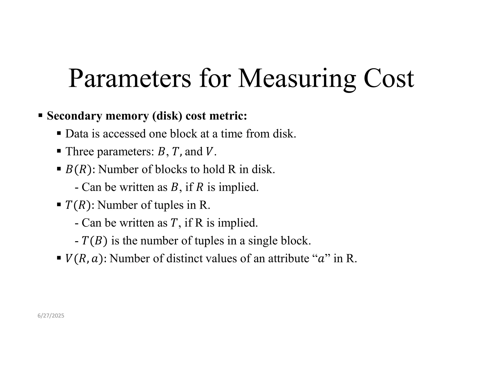
Parameters for Measuring Cost  Secondary memory (disk) cost metric:  Data is accessed one block at a time from disk.  Three parameters: , and .  Number of blocks to hold R in disk. - Can be written as , if is implied.  Number of tuples in R. - Can be written as , if R is implied. - is the number of tuples in a single block.  Number of distinct values of an attribute “ ” in R. 6/27/2025

I/O Cost for Scan Operation  Cost of table-scan:  Number of disk I/Os is [irrespective of clustered vs. non-clustered]  Cost of index-scan:  Number of disk I/Os is approximately:  [If is clustered index]  [If is not clustered index]  Cost  Typically, we assume all relations are clustered index [unless otherwise stated]. 6/27/2025

I/O Cost for Scan Operation  Cost of sort-scan:  If is a clustered-index - Perform an index-scan to read [already sorted] - Cost =  If fits in main memory: - Read into memory. - Perform an in-memory sort on . - Cost =  If does not fit in main memory: - Cost > [algorithm discussed later] 6/27/2025

I/O Cost for Index-scan Operation  Cost of index-scan:  Read the index first: blocks read.  Read the blocks of : blocks read. [assuming clustered-index]  Total = [B(I) << B(R)] = [If  Not useful when full is required.  Useful when only a part of is required.  Only relevant blocks of are retrieved. 6/27/2025

Iterators for Physical Plan Operators  Iterators are implemented for physical operators:  Returns result of operator one tuple at a time.  Iterators have following three methods:  Open: initializes data structure for getting blocks and tuples.  Getnext: returns the next tuple in the result.  Close: clears data structure. 6/27/2025

Types of algorithms for physical plan operators  One pass algorithms  Involve reading each data blok only once from disk.  Require at least one argument to fit in main memory.  Two-pass algorithms  Relations are too large to fit in main memory.  Involve each block two times read from disk.  Read first time from disk, process in some way, write to disk, and reads a second time from disk. 6/27/2025

Types of algorithms for physical plan operators  Many-pass algorithms  Data has no limit.  Involve three or more passes.  Each data block is read three or more times from the disk 6/27/2025

Types of Physical Plan Operations  Tuple-at-a-time, Unary Operations  Operations require only one-tuple at a time for producing outputs.  Example operators:  Selection:  Projection:  Do not require entire relation in memory at once.  Read one block at a time in a main-memory buffer and produce the output. 6/27/2025

Types of Physical Plan Operations  Full-relation, Unary Operations  Operation requires full-relation access to produce outputs.  Example operators:  Gamma: (grouping operator)  Delta: (duplicate-elimination operator)  Require all or most of the tuples in memory at once. [ Why? ]  One pass algorithms can be used only if fits in . 6/27/2025

Types of Physical Plan Operations  Full-relation, Binary Operation  Operation requires full-relation access to produce outputs.  Example operators:  Union:  Intersection:  Natural join:  Cartesian product (cross join):  One pass algorithm may be used if at least one argument fits in main- memory. 6/27/2025

One pass Algorithm for Tuple-at-a-time Operation  Relational algebra operations: and  Approach:  Read blocks one at a time in an input buffer.  Perform the operation on each tuple and move selected tuple to the output buffer.  Requirement: regardless of .  I/O Cost:  if is clustered index or table-scan is used.  if is not clustered index and index-scan is used. [very expensive]  Exception: For predicate-based selection for which an index is available, use index to retrieve a subset of .  Cost of index-scan: < B(R) [index-seek] 6/27/2025

One-pass Algorithm for Unary, Full-Relation Operation  Relational algebra operation: [Duplicate elimination]  Use one memory block to hold one block of  Use remaining buffers to hold output tuples [single copy of each tuple of ].  Algorithm:  For each tuple in retrieved block:  If it is already in output tuples, then discard (don’t copy to output buffer).  Otherwise copy to output block. 6/27/2025

One-pass Algorithm for Unary, Full-Relation Operation  Cost of checking whether a tuple already exists in output list:  if checking required proportional to [size of output], total time = for duplicate checking.  if used a hash table with a large number of buckets for output list.  Requirement: . [size of R with unique tuples should fit in M-1 buffers ]  What if ?  Outputs doesn't fit in main memory.  Output must be moved to disk back and forth, resulting in thrashing.  Increases I/O cost for duplicate checking. 6/27/2025

One-pass Algorithm for Unary, Full-Relation Operation  Grouping operation:  Involves zero or more grouping attribute  One or more aggregate attributes  Algorithm:  If we create one entry for each group in main memory: - Scan the blocks of one at a time. - For each tuple, find the entry corresponding to the tuple and update aggregated result of the group. - For aggregate, record the and seen so far. - For aggregation, add one to accumulated value. - For aggregation, add the value of a to the accumulated sums. - For , use two accumulations, and 6/27/2025

One-pass algorithm for Unary, Full-Relation Operation  Result generation:  When all tuples of are read.  Output contains one entry for each group from the main memory.  Requirement:  Efficient data structure for finding group entry for a tuple.  Hash tables or balanced trees can be used.  Number of disk I/Os:  Memory buffers requirement: . [Size of R with unique rows should fit in M-1 buffers] 6/27/2025

Binary Operations: Bag Union  Bag union:  R and S are bags. Union keeps all tuples.  Algorithm:  First copy every tuple of  Then copy every tuple of  Number of disk I/Os:  Number of memory buffers required: suffices. [ no need to store; pipelining allows outputs one tuple-at-a-time ] 6/27/2025

Binary Operations: Set Union  Set union:  R and S are sets.  Union keeps one copy of each common tuple occurring in both R and S. 6/27/2025

Binary Operations: Set Union  Algorithm for :  Assume  First read and copy in main memory buffers, build a main memory data structure on search key [ entire tuple is the search key ]  Copy all tuples of into output.  Retrieve one block of at a time in main memory buffer. For each tuple of , check if it is also in [ using main memory data structure on search key ]  If it is not in , copy it to output.  Efficient data structure is required for storing 𝐵(𝑆) in main memory so that check operation can be done efficiently.  If it is in , don’t copy. 6/27/2025

Binary Operations: Set Union  Set union:  Number of disk I/Os required:  Number of memory buffers required: . [ At least one of R and S must fit in M-1 buffers ] 6/27/2025

Binary Operations: Set Intersection  Set Intersection: .  and are sets. Intersection keeps only common tuples of R and S.  Algorithm:  Assume .  Read into main memory buffers, build a search data structure [key is full tuple]  Read each block of For each tuple of , check if it is also in [using main memory data structure on search key to check]  If it is in , copy it to output.  If it is not in , don’t copy.  Number of disk I/Os required: .  Number of memory buffers required: . 6/27/2025

Binary Operations: Set Difference  Set Difference: .  and are sets.  Keeps tuples of R that are not in S.  Algorithm:  Assume  Read into main memory buffers, build a search data structure [search key is full tuple]  Read each block of For each tuple of , check if it is also in  If it is not in , copy it to output.  If it is in , don’t copy to output.  Number of disk I/Os required:  Number of memory buffers required: [ At least one of R and S must fit in M-1 buffers ] 6/27/2025

Binary Operations: Bag Intersection  Bag intersection: .  R and S are bags.  Bags allow multiples copies of the same tuple.  Also known as multi-sets.  An element appears in the intersection the minimum of the number of times it appears in either. 6/27/2025

Binary Operations: Bag Intersection  Algorithm for bag intersection:  Assume  Read into main memory buffers, build a search data structure [key is full tuple] along with a count value.  Main memory stores only unique tuples of .  Count is the number of times tuple occurs in .  Read each block of For each tuple of , check if it is also in and check the count:  If count is positive, decrease by one, and copy the tuple to the output.  If count is zero, no action is required.  Number of disk I/Os required:  Number of memory buffers required: 6/27/2025

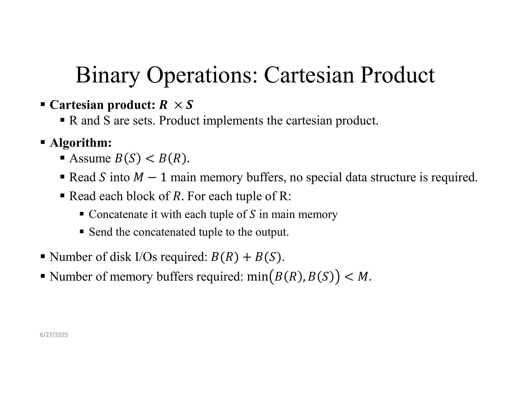
Binary Operations: Cartesian Product  Cartesian product:  R and S are sets. Product implements the cartesian product.  Algorithm:  Assume  Read into main memory buffers, no special data structure is required.  Read each block of For each tuple of R:  Concatenate it with each tuple of in main memory  Send the concatenated tuple to the output.  Number of disk I/Os required: .  Number of memory buffers required: 6/27/2025

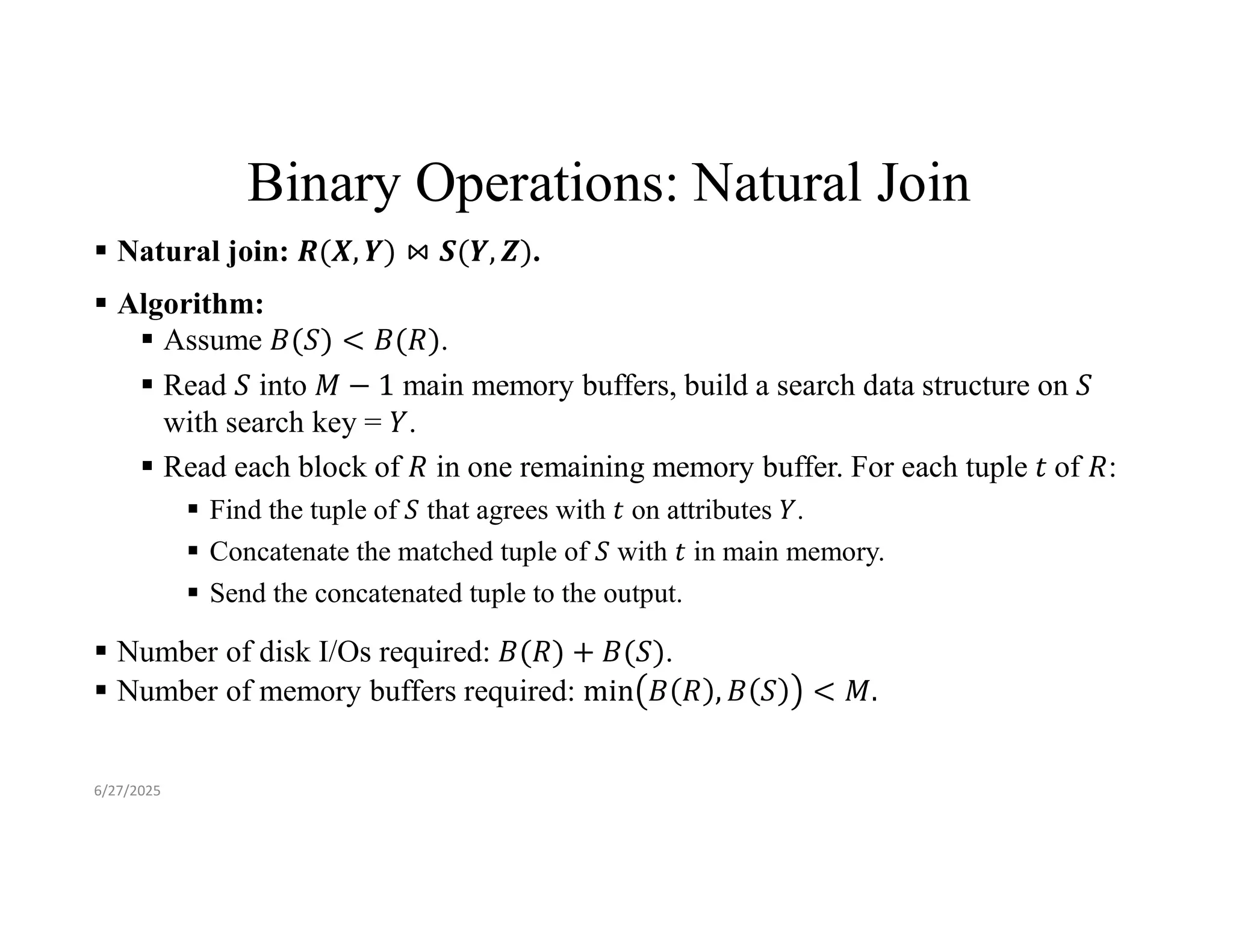
Binary Operations: Natural Join  Natural join: .  Algorithm:  Assume .  Read into main memory buffers, build a search data structure on with search key = .  Read each block of in one remaining memory buffer. For each tuple of :  Find the tuple of that agrees with on attributes .  Concatenate the matched tuple of with in main memory.  Send the concatenated tuple to the output.  Number of disk I/Os required: .  Number of memory buffers required: 6/27/2025

DBMS Query Optimization along with algorithms

More Related Content

Similar to DBMS Query Optimization along with algorithms

Recently uploaded

DBMS Query Optimization along with algorithms