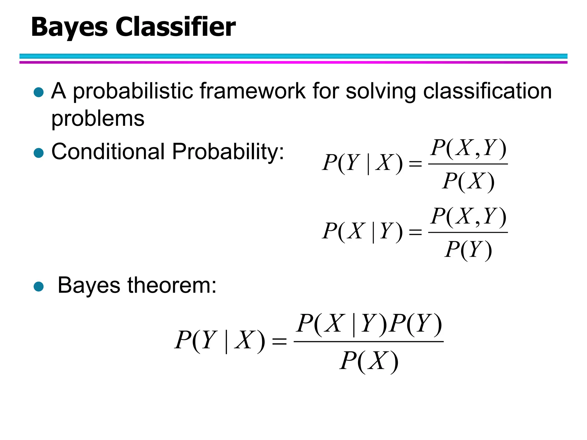
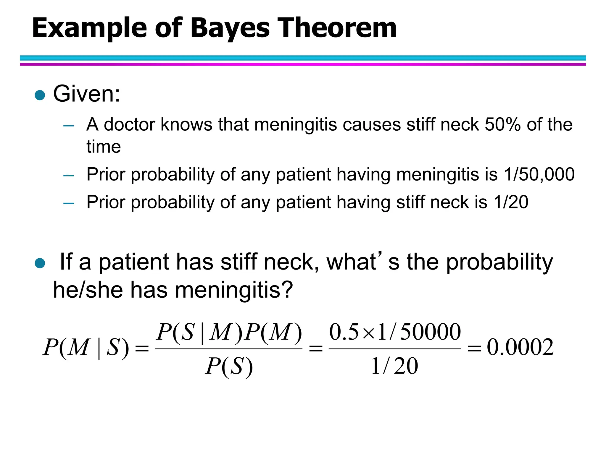
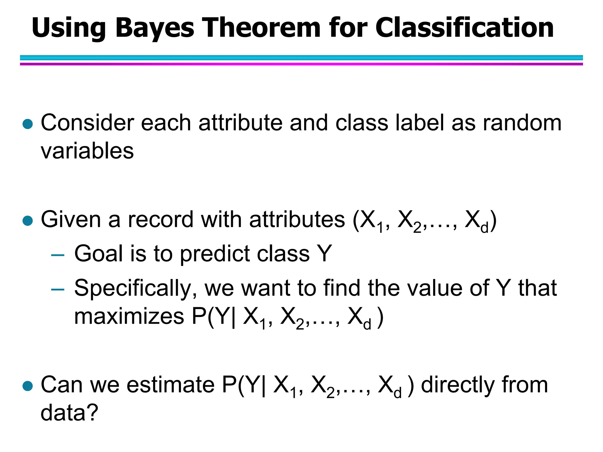
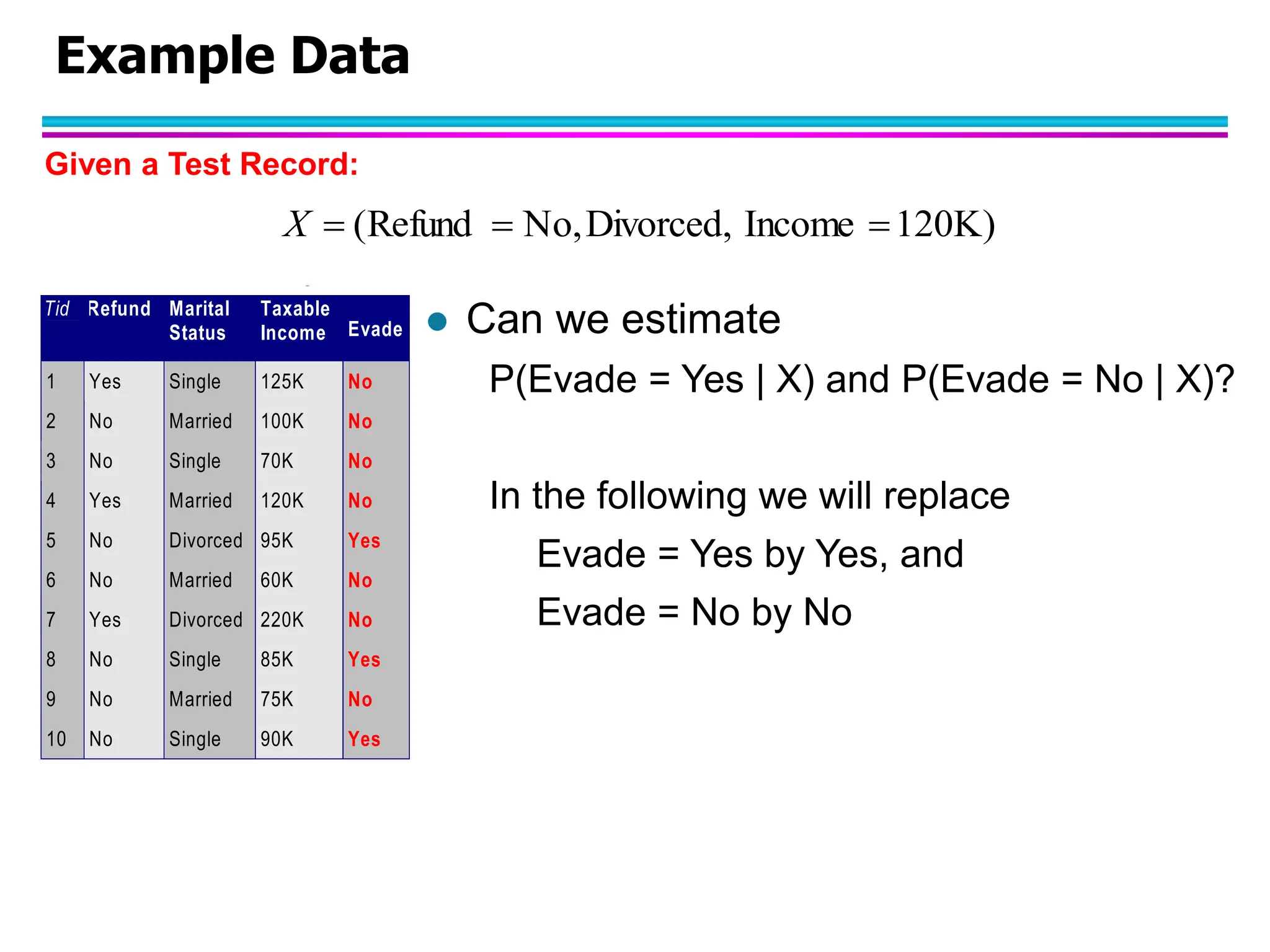
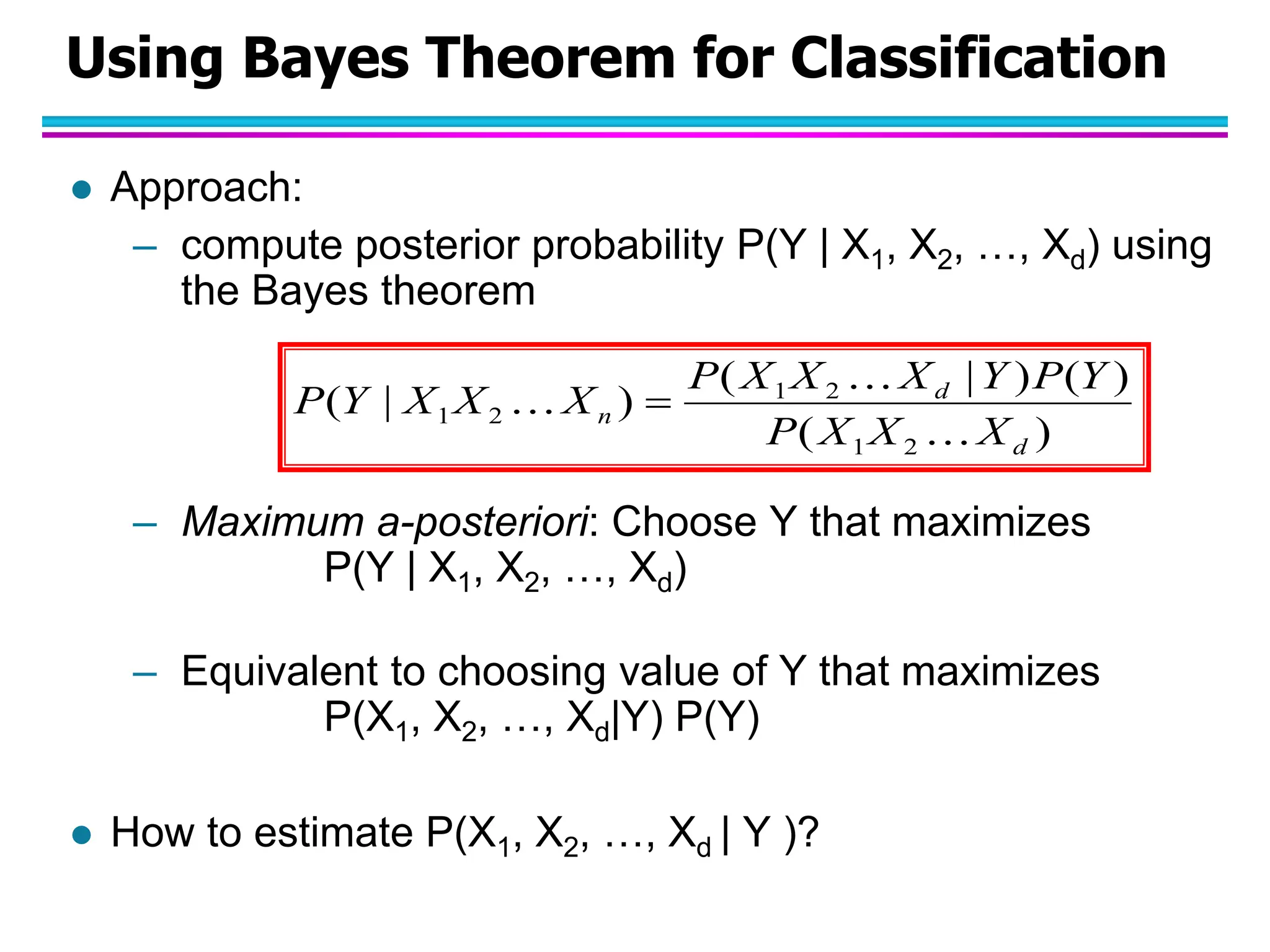
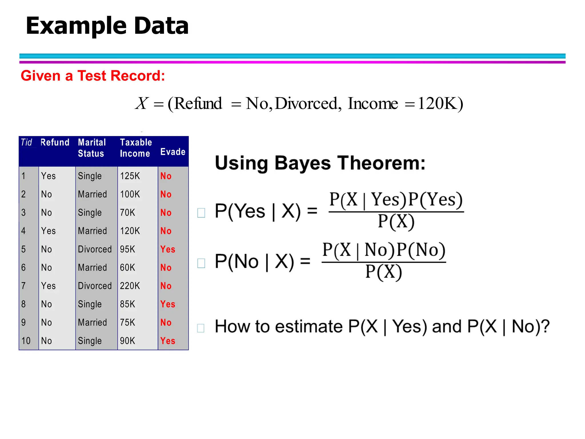
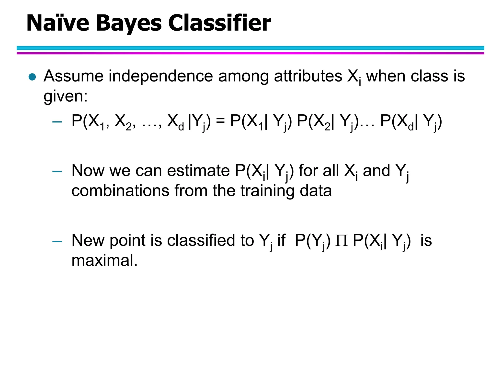
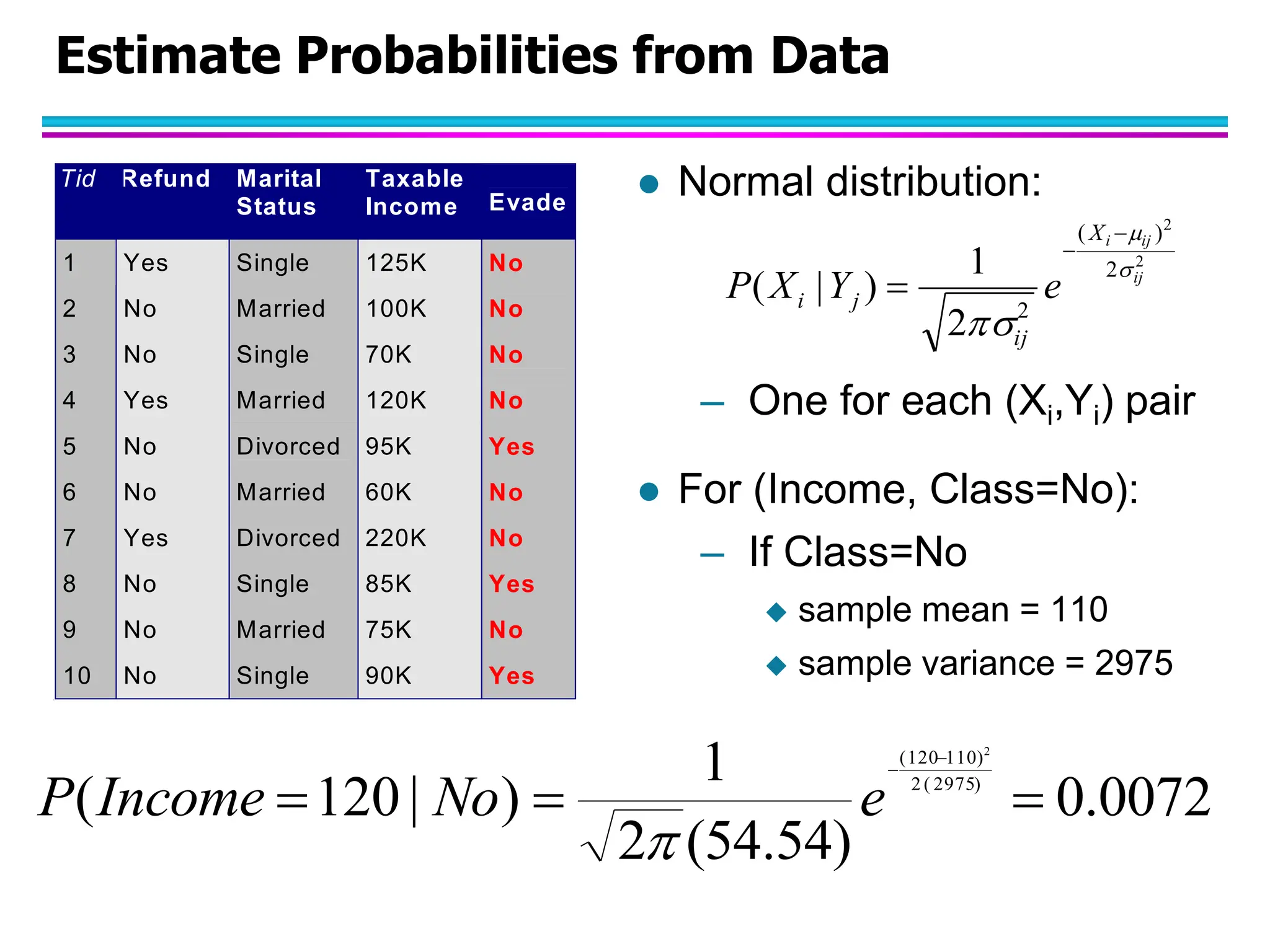
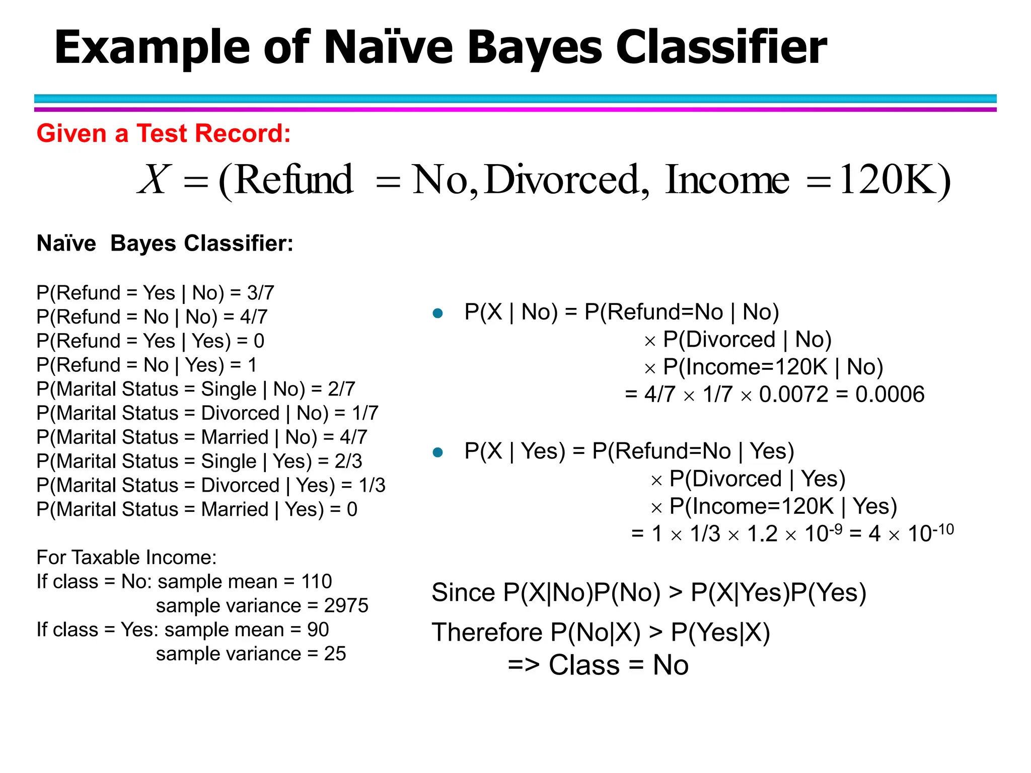
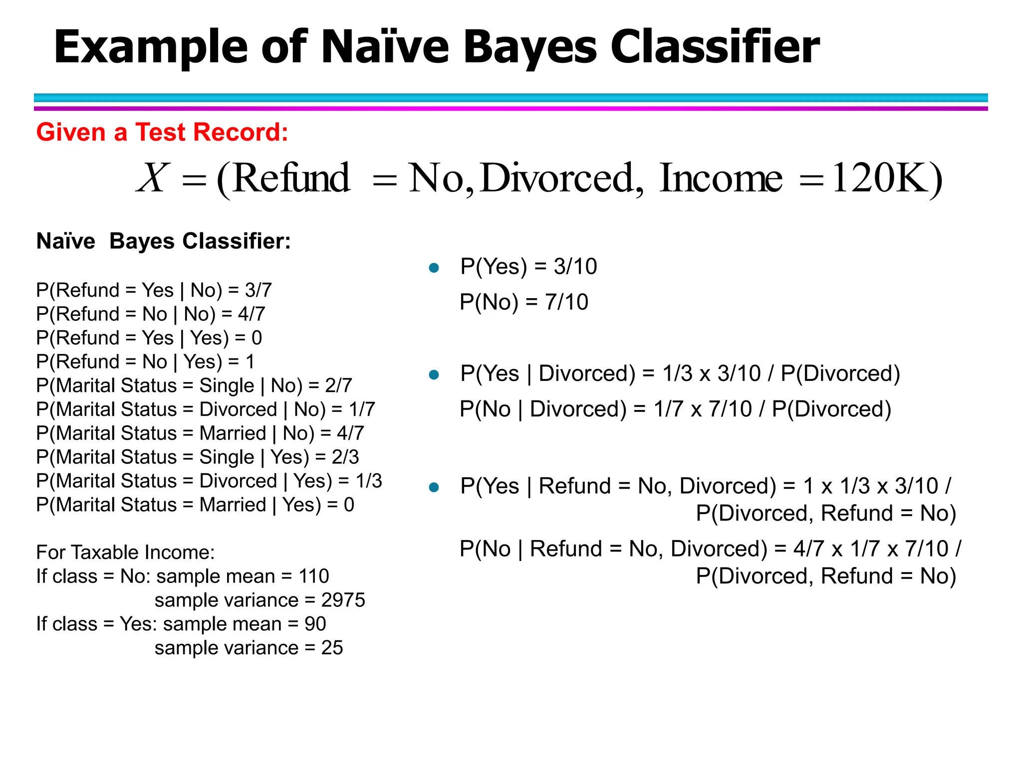
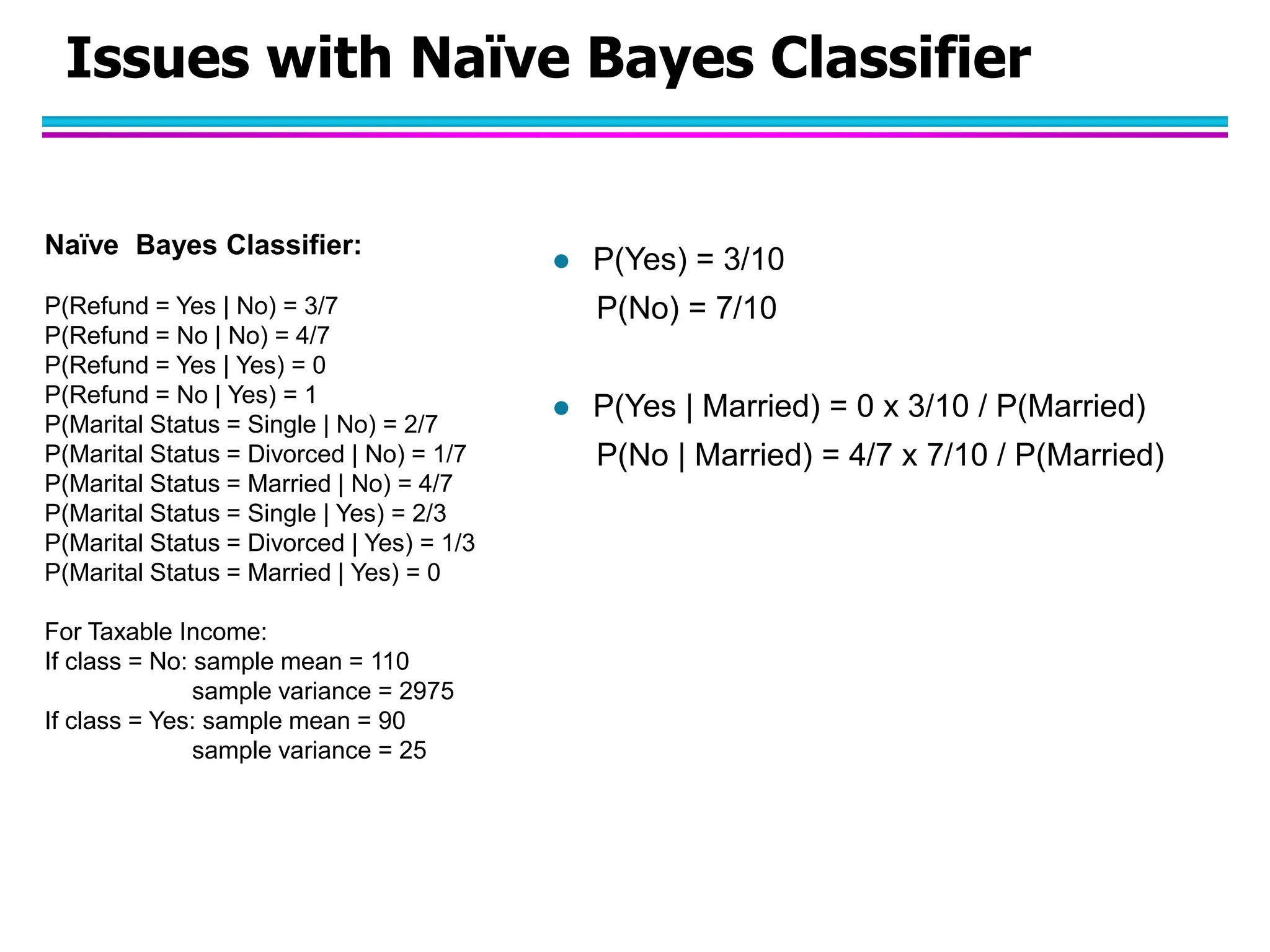
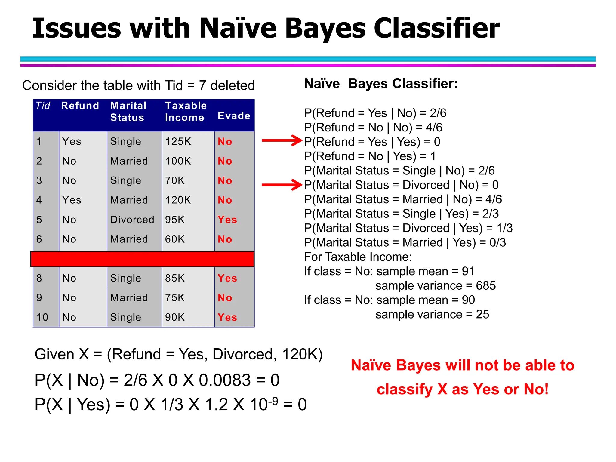
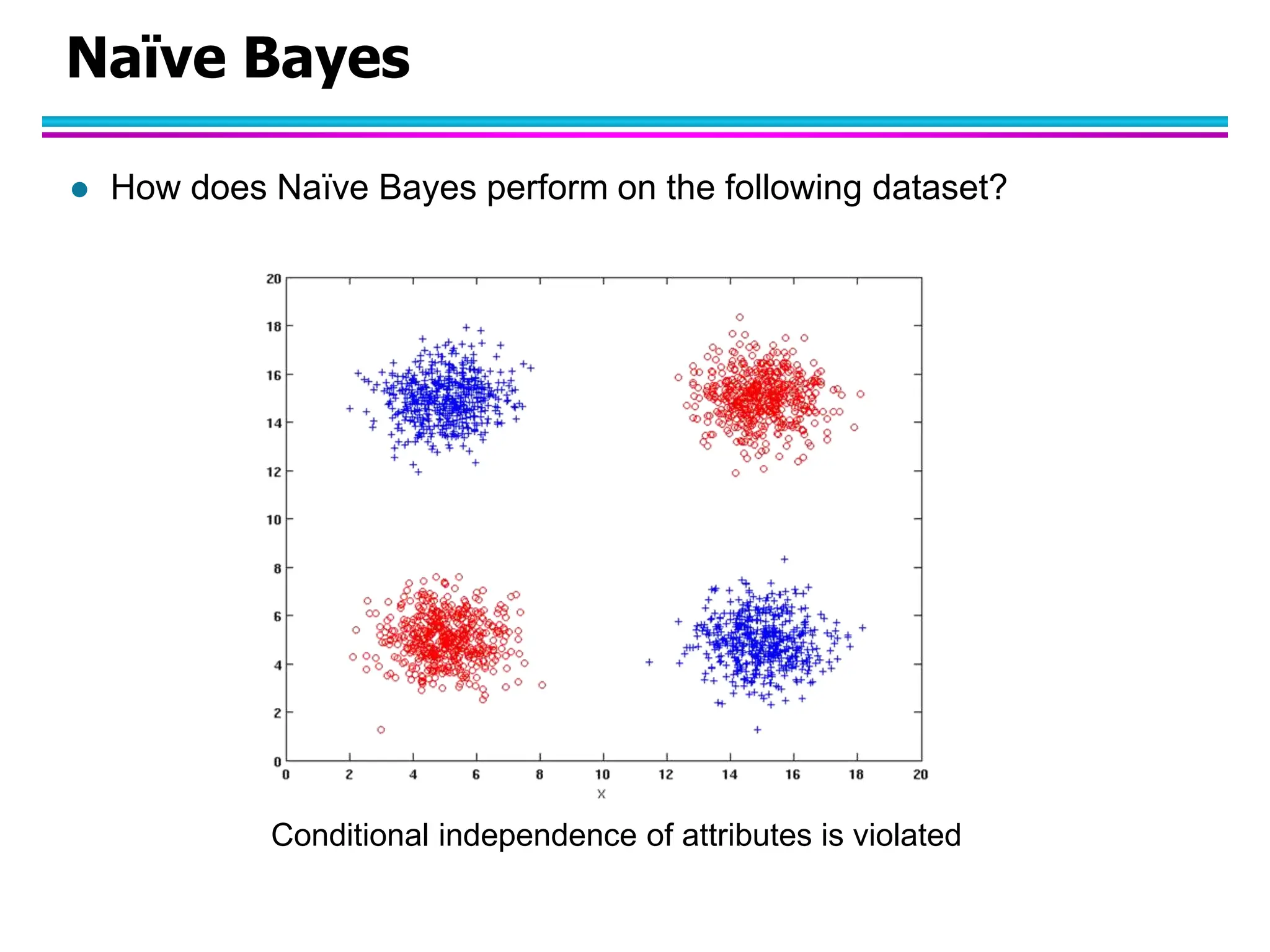
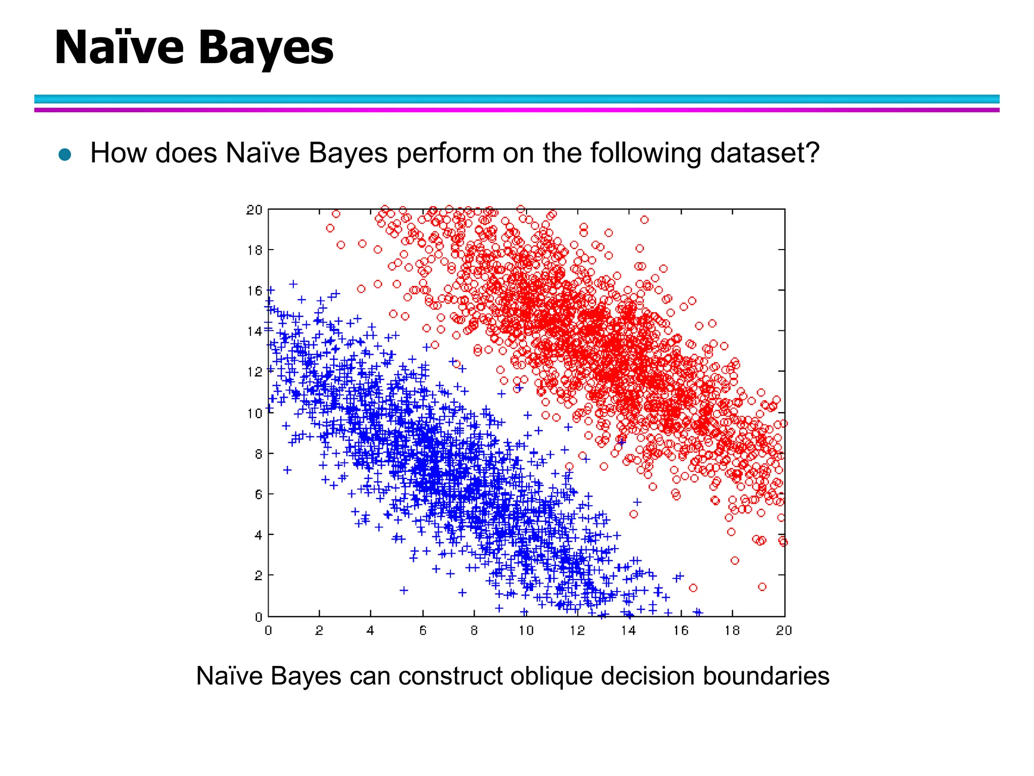
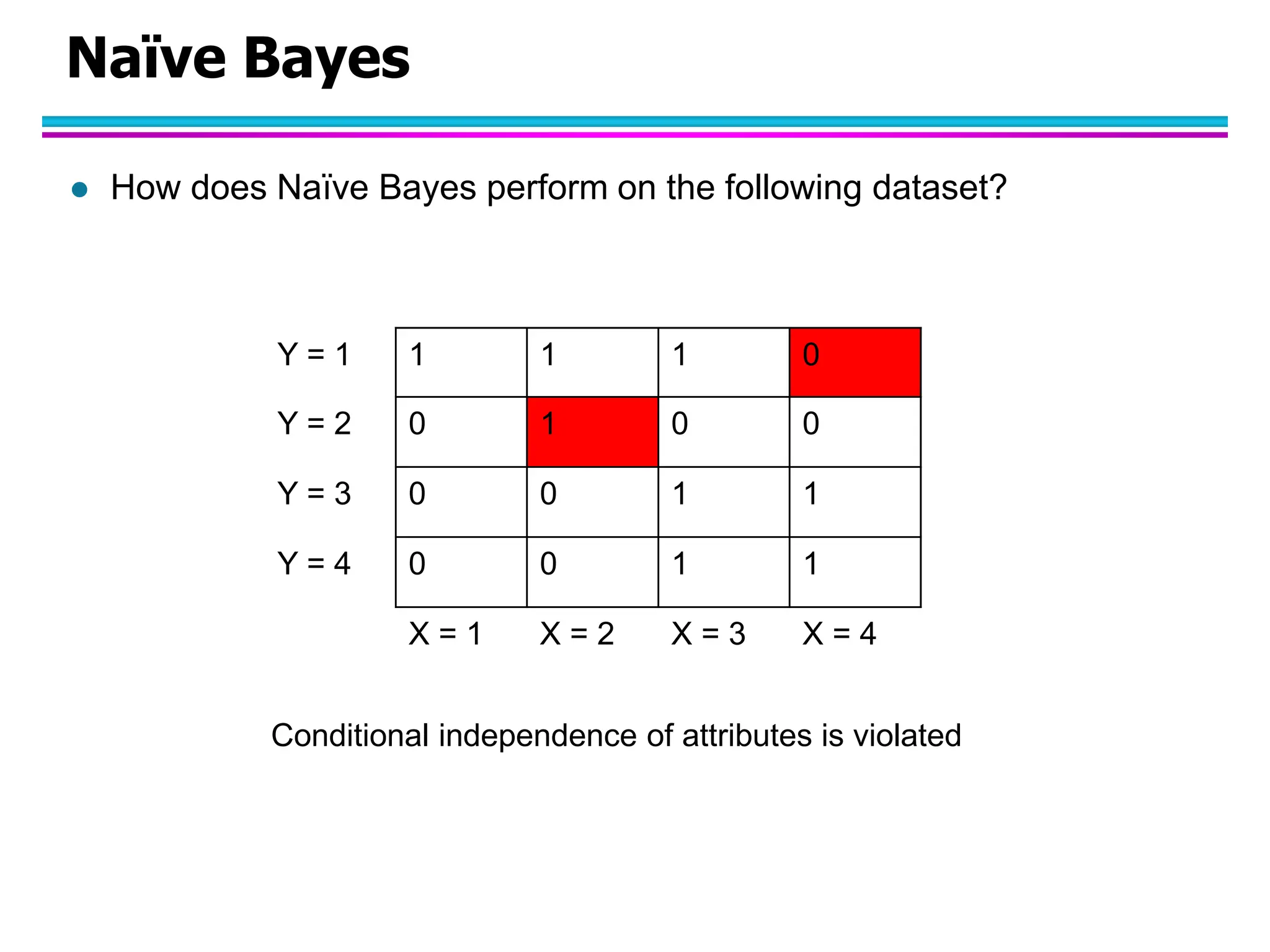
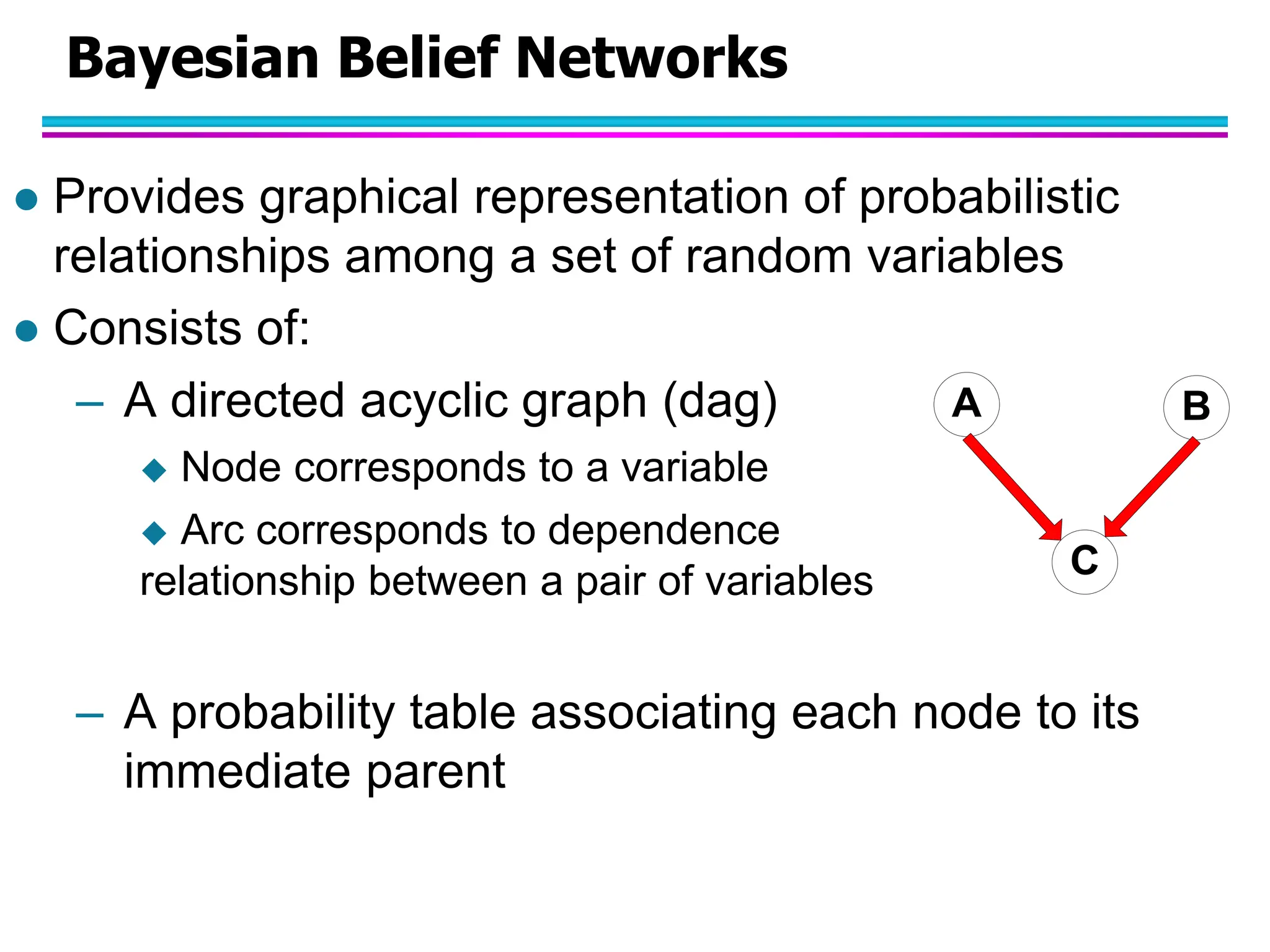
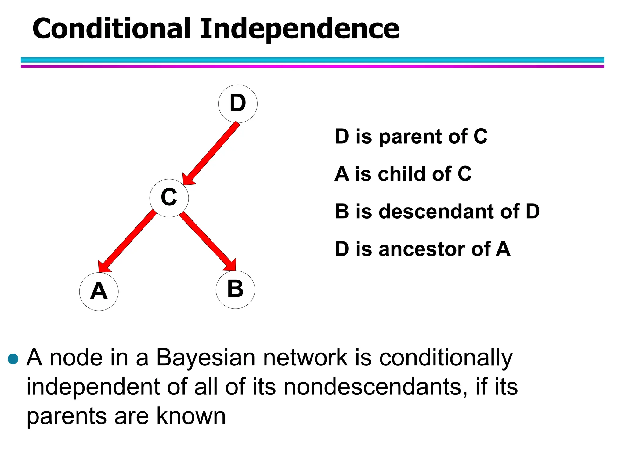
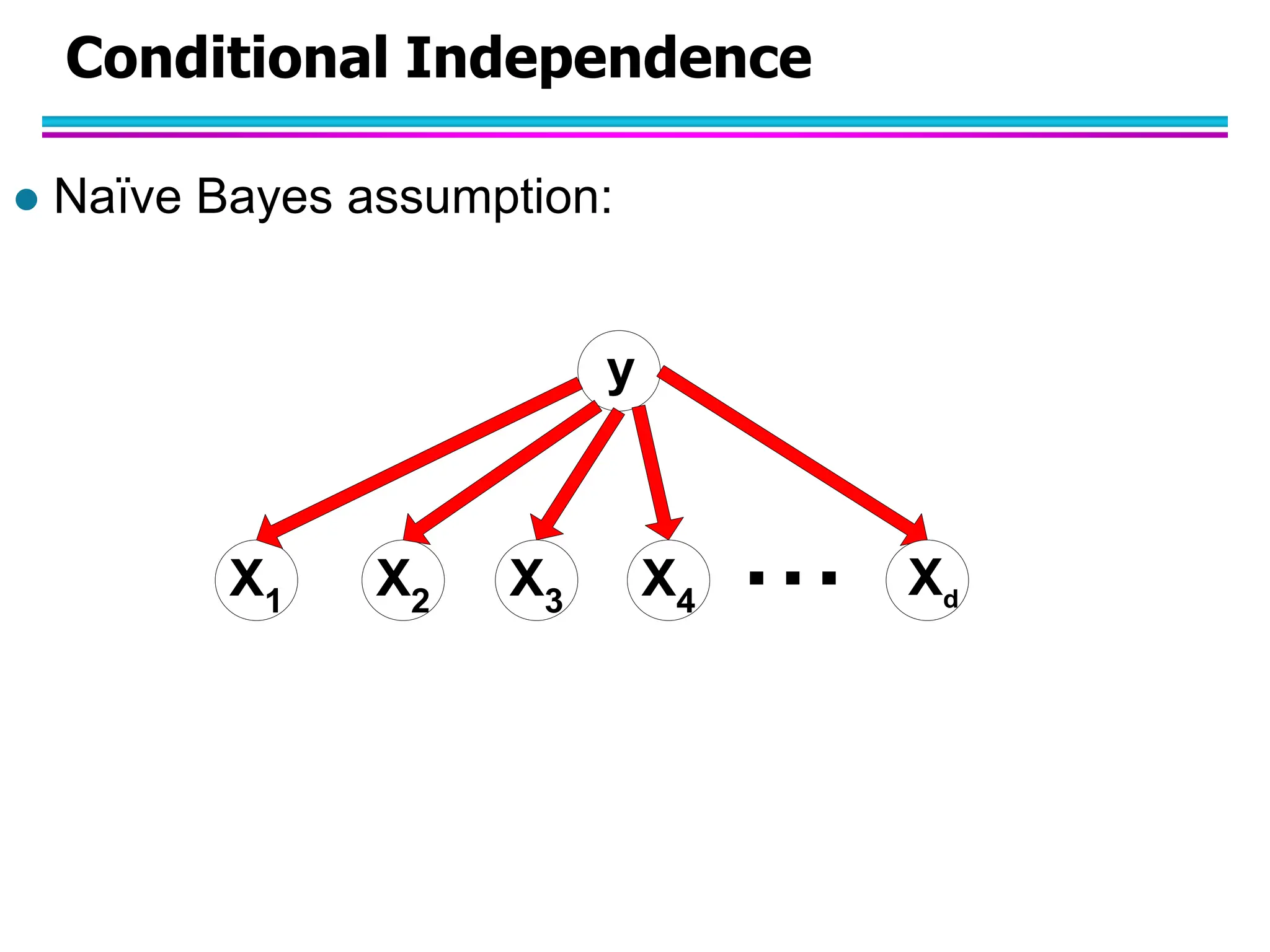
introduction to basic classification methods

Bayesian Classifiers Data Mining Classification: Alternative Techniques

Bayes Classifier  A probabilistic framework for solving classification problems  Conditional Probability:  Bayes theorem: ) ( ) ( ) | ( ) | ( X P Y P Y X P X Y P  ) ( ) , ( ) | ( ) ( ) , ( ) | ( Y P Y X P Y X P X P Y X P X Y P  

Example of Bayes Theorem  Given: – A doctor knows that meningitis causes stiff neck 50% of the time – Prior probability of any patient having meningitis is 1/50,000 – Prior probability of any patient having stiff neck is 1/20  If a patient has stiff neck, what’s the probability he/she has meningitis? 0002 . 0 20 / 1 50000 / 1 5 . 0 ) ( ) ( ) | ( ) | (     S P M P M S P S M P

Using Bayes Theorem for Classification  Consider each attribute and class label as random variables  Given a record with attributes (X1, X2,…, Xd) – Goal is to predict class Y – Specifically, we want to find the value of Y that maximizes P(Y| X1, X2,…, Xd )  Can we estimate P(Y| X1, X2,…, Xd ) directly from data?

Example Data Tid Refund Marital Status Taxable Income Evade 1 Yes Single 125K No 2 No Married 100K No 3 No Single 70K No 4 Yes Married 120K No 5 No Divorced 95K Yes 6 No Married 60K No 7 Yes Divorced 220K No 8 No Single 85K Yes 9 No Married 75K No 10 No Single 90K Yes 10 categorical categorical continuous class 120K) Income Divorced, No, Refund (    X Given a Test Record:  Can we estimate P(Evade = Yes | X) and P(Evade = No | X)? In the following we will replace Evade = Yes by Yes, and Evade = No by No

Using Bayes Theorem for Classification  Approach: – compute posterior probability P(Y | X1, X2, …, Xd) using the Bayes theorem – Maximum a-posteriori: Choose Y that maximizes P(Y | X1, X2, …, Xd) – Equivalent to choosing value of Y that maximizes P(X1, X2, …, Xd|Y) P(Y)  How to estimate P(X1, X2, …, Xd | Y )? ) ( ) ( ) | ( ) | ( 2 1 2 1 2 1 d d n X X X P Y P Y X X X P X X X Y P    

Example Data Tid Refund Marital Status Taxable Income Evade 1 Yes Single 125K No 2 No Married 100K No 3 No Single 70K No 4 Yes Married 120K No 5 No Divorced 95K Yes 6 No Married 60K No 7 Yes Divorced 220K No 8 No Single 85K Yes 9 No Married 75K No 10 No Single 90K Yes 10 categorical categorical continuous class 120K) Income Divorced, No, Refund (    X Given a Test Record:

Conditional Independence  X and Y are conditionally independent given Z if P(X|YZ) = P(X|Z)  Example: Arm length and reading skills – Young child has shorter arm length and limited reading skills, compared to adults – If age is fixed, no apparent relationship between arm length and reading skills – Arm length and reading skills are conditionally independent given age

Naïve Bayes on Example Data Tid Refund Marital Status Taxable Income Evade 1 Yes Single 125K No 2 No Married 100K No 3 No Single 70K No 4 Yes Married 120K No 5 No Divorced 95K Yes 6 No Married 60K No 7 Yes Divorced 220K No 8 No Single 85K Yes 9 No Married 75K No 10 No Single 90K Yes 10 categorical categorical continuous class 120K) Income Divorced, No, Refund (    X Given a Test Record:  P(X | Yes) = P(Refund = No | Yes) x P(Divorced | Yes) x P(Income = 120K | Yes)  P(X | No) = P(Refund = No | No) x P(Divorced | No) x P(Income = 120K | No)

Estimate Probabilities from Data  Class: P(Y) = Nc/N – e.g., P(No) = 7/10, P(Yes) = 3/10  For categorical attributes: P(Xi | Yk) = |Xik|/ Nc – where |Xik| is number of instances having attribute value Xi and belonging to class Yk – Examples: P(Status=Married|No) = 4/7 P(Refund=Yes|Yes)=0 k Tid Refund Marital Status Taxable Income Evade 1 Yes Single 125K No 2 No Married 100K No 3 No Single 70K No 4 Yes Married 120K No 5 No Divorced 95K Yes 6 No Married 60K No 7 Yes Divorced 220K No 8 No Single 85K Yes 9 No Married 75K No 10 No Single 90K Yes 10 categorical categorical continuous class

Estimate Probabilities from Data  For continuous attributes: – Discretization: Partition the range into bins:  Replace continuous value with bin value – Attribute changed from continuous to ordinal – Probability density estimation:  Assume attribute follows a normal distribution  Use data to estimate parameters of distribution (e.g., mean and standard deviation)  Once probability distribution is known, use it to estimate the conditional probability P(Xi|Y) k

Estimate Probabilities from Data  Normal distribution: – One for each (Xi,Yi) pair  For (Income, Class=No): – If Class=No  sample mean = 110  sample variance = 2975 Tid Refund Marital Status Taxable Income Evade 1 Yes Single 125K No 2 No Married 100K No 3 No Single 70K No 4 Yes Married 120K No 5 No Divorced 95K Yes 6 No Married 60K No 7 Yes Divorced 220K No 8 No Single 85K Yes 9 No Married 75K No 10 No Single 90K Yes 10 categorical categorical continuous class 2 2 2 ) ( 2 2 1 ) | ( ij ij i X ij j i e Y X P       0072 . 0 ) 54 . 54 ( 2 1 ) | 120 ( ) 2975 ( 2 ) 110 120 ( 2      e No Income P 

Example of Naïve Bayes Classifier 120K) Income Divorced, No, Refund (    X  P(Yes) = 3/10 P(No) = 7/10  P(Yes | Divorced) = 1/3 x 3/10 / P(Divorced) P(No | Divorced) = 1/7 x 7/10 / P(Divorced)  P(Yes | Refund = No, Divorced) = 1 x 1/3 x 3/10 / P(Divorced, Refund = No) P(No | Refund = No, Divorced) = 4/7 x 1/7 x 7/10 / P(Divorced, Refund = No) Given a Test Record: Naïve Bayes Classifier: P(Refund = Yes | No) = 3/7 P(Refund = No | No) = 4/7 P(Refund = Yes | Yes) = 0 P(Refund = No | Yes) = 1 P(Marital Status = Single | No) = 2/7 P(Marital Status = Divorced | No) = 1/7 P(Marital Status = Married | No) = 4/7 P(Marital Status = Single | Yes) = 2/3 P(Marital Status = Divorced | Yes) = 1/3 P(Marital Status = Married | Yes) = 0 For Taxable Income: If class = No: sample mean = 110 sample variance = 2975 If class = Yes: sample mean = 90 sample variance = 25

Issues with Naïve Bayes Classifier  P(Yes) = 3/10 P(No) = 7/10  P(Yes | Married) = 0 x 3/10 / P(Married) P(No | Married) = 4/7 x 7/10 / P(Married) Naïve Bayes Classifier: P(Refund = Yes | No) = 3/7 P(Refund = No | No) = 4/7 P(Refund = Yes | Yes) = 0 P(Refund = No | Yes) = 1 P(Marital Status = Single | No) = 2/7 P(Marital Status = Divorced | No) = 1/7 P(Marital Status = Married | No) = 4/7 P(Marital Status = Single | Yes) = 2/3 P(Marital Status = Divorced | Yes) = 1/3 P(Marital Status = Married | Yes) = 0 For Taxable Income: If class = No: sample mean = 110 sample variance = 2975 If class = Yes: sample mean = 90 sample variance = 25

Issues with Naïve Bayes Classifier Tid Refund Marital Status Taxable Income Evade 1 Yes Single 125K No 2 No Married 100K No 3 No Single 70K No 4 Yes Married 120K No 5 No Divorced 95K Yes 6 No Married 60K No 7 Yes Divorced 220K No 8 No Single 85K Yes 9 No Married 75K No 10 No Single 90K Yes 10 categorical categorical continuous class Naïve Bayes Classifier: P(Refund = Yes | No) = 2/6 P(Refund = No | No) = 4/6 P(Refund = Yes | Yes) = 0 P(Refund = No | Yes) = 1 P(Marital Status = Single | No) = 2/6 P(Marital Status = Divorced | No) = 0 P(Marital Status = Married | No) = 4/6 P(Marital Status = Single | Yes) = 2/3 P(Marital Status = Divorced | Yes) = 1/3 P(Marital Status = Married | Yes) = 0/3 For Taxable Income: If class = No: sample mean = 91 sample variance = 685 If class = No: sample mean = 90 sample variance = 25 Consider the table with Tid = 7 deleted Given X = (Refund = Yes, Divorced, 120K) P(X | No) = 2/6 X 0 X 0.0083 = 0 P(X | Yes) = 0 X 1/3 X 1.2 X 10-9 = 0 Naïve Bayes will not be able to classify X as Yes or No!

Issues with Naïve Bayes Classifier  If one of the conditional probabilities is zero, then the entire expression becomes zero  Need to use other estimates of conditional probabilities than simple fractions  Probability estimation: m N mp N C A P c N N C A P N N C A P c ic i c ic i c ic i        ) | ( : estimate - m 1 ) | ( : Laplace ) | ( : Original c: number of classes p: prior probability of the class m: parameter Nc: number of instances in the class Nic: number of instances having attribute value Ai in class c

Example of Naïve Bayes Classifier Name Give Birth Can Fly Live in Water Have Legs Class human yes no no yes mammals python no no no no non-mammals salmon no no yes no non-mammals whale yes no yes no mammals frog no no sometimes yes non-mammals komodo no no no yes non-mammals bat yes yes no yes mammals pigeon no yes no yes non-mammals cat yes no no yes mammals leopard shark yes no yes no non-mammals turtle no no sometimes yes non-mammals penguin no no sometimes yes non-mammals porcupine yes no no yes mammals eel no no yes no non-mammals salamander no no sometimes yes non-mammals gila monster no no no yes non-mammals platypus no no no yes mammals owl no yes no yes non-mammals dolphin yes no yes no mammals eagle no yes no yes non-mammals Give Birth Can Fly Live in Water Have Legs Class yes no yes no ? 0027 . 0 20 13 004 . 0 ) ( ) | ( 021 . 0 20 7 06 . 0 ) ( ) | ( 0042 . 0 13 4 13 3 13 10 13 1 ) | ( 06 . 0 7 2 7 2 7 6 7 6 ) | (                 N P N A P M P M A P N A P M A P A: attributes M: mammals N: non-mammals P(A|M)P(M) > P(A|N)P(N) => Mammals

Naïve Bayes (Summary)  Robust to isolated noise points  Handle missing values by ignoring the instance during probability estimate calculations  Robust to irrelevant attributes  Independence assumption may not hold for some attributes – Use other techniques such as Bayesian Belief Networks (BBN)

Naïve Bayes  How does Naïve Bayes perform on the following dataset? Conditional independence of attributes is violated

Naïve Bayes  How does Naïve Bayes perform on the following dataset? Naïve Bayes can construct oblique decision boundaries

Naïve Bayes  How does Naïve Bayes perform on the following dataset? Y = 1 1 1 1 0 Y = 2 0 1 0 0 Y = 3 0 0 1 1 Y = 4 0 0 1 1 X = 1 X = 2 X = 3 X = 4 Y = 1 1 1 1 0 Y = 2 0 1 0 0 Y = 3 0 0 1 1 Y = 4 0 0 1 1 X = 1 X = 2 X = 3 X = 4 Conditional independence of attributes is violated

Bayesian Belief Networks A B C  Provides graphical representation of probabilistic relationships among a set of random variables  Consists of: – A directed acyclic graph (dag)  Node corresponds to a variable  Arc corresponds to dependence relationship between a pair of variables – A probability table associating each node to its immediate parent

Conditional Independence A B C D  A node in a Bayesian network is conditionally independent of all of its nondescendants, if its parents are known D is parent of C A is child of C B is descendant of D D is ancestor of A

Conditional Independence ... X1 X2 X3 X4 y Xd  Naïve Bayes assumption:

Probability Tables Y X  If X does not have any parents, table contains prior probability P(X)  If X has only one parent (Y), table contains conditional probability P(X|Y)  If X has multiple parents (Y1, Y2,…, Yk), table contains conditional probability P(X|Y1, Y2,…, Yk)

Example of Bayesian Belief Network Exercise Diet Heart Disease Chest Pain Blood Pressure Exercise=Yes 0.7 Exercise=No 0.3 Diet=Healthy 0.25 Diet=Unhealthy 0.75 E=Healthy D=Yes E=Healthy D=No E=Unhealthy D=Yes E=Unhealthy D=No HD=Yes 0.25 0.45 0.55 0.75 HD=No 0.75 0.55 0.45 0.25 HD=Yes HD=No CP=Yes 0.8 0.01 CP=No 0.2 0.99 HD=Yes HD=No BP=High 0.85 0.2 BP=Low 0.15 0.8

introduction to basic classification methods

More Related Content

Similar to introduction to basic classification methods

More from Radhika R

Recently uploaded

introduction to basic classification methods