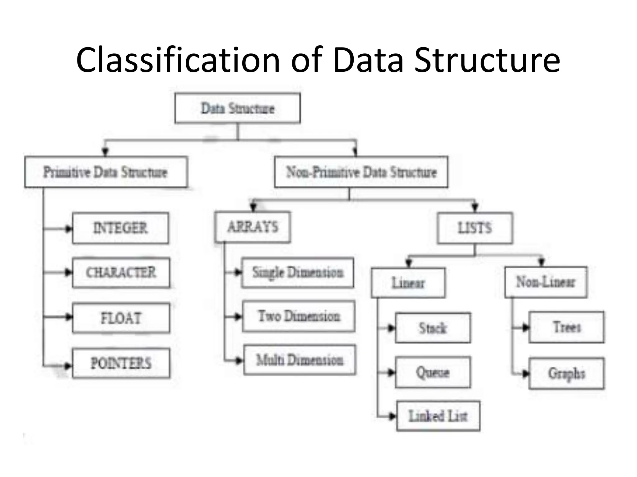
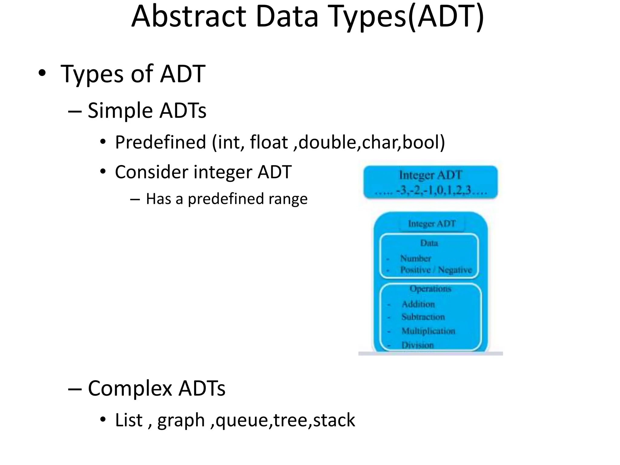
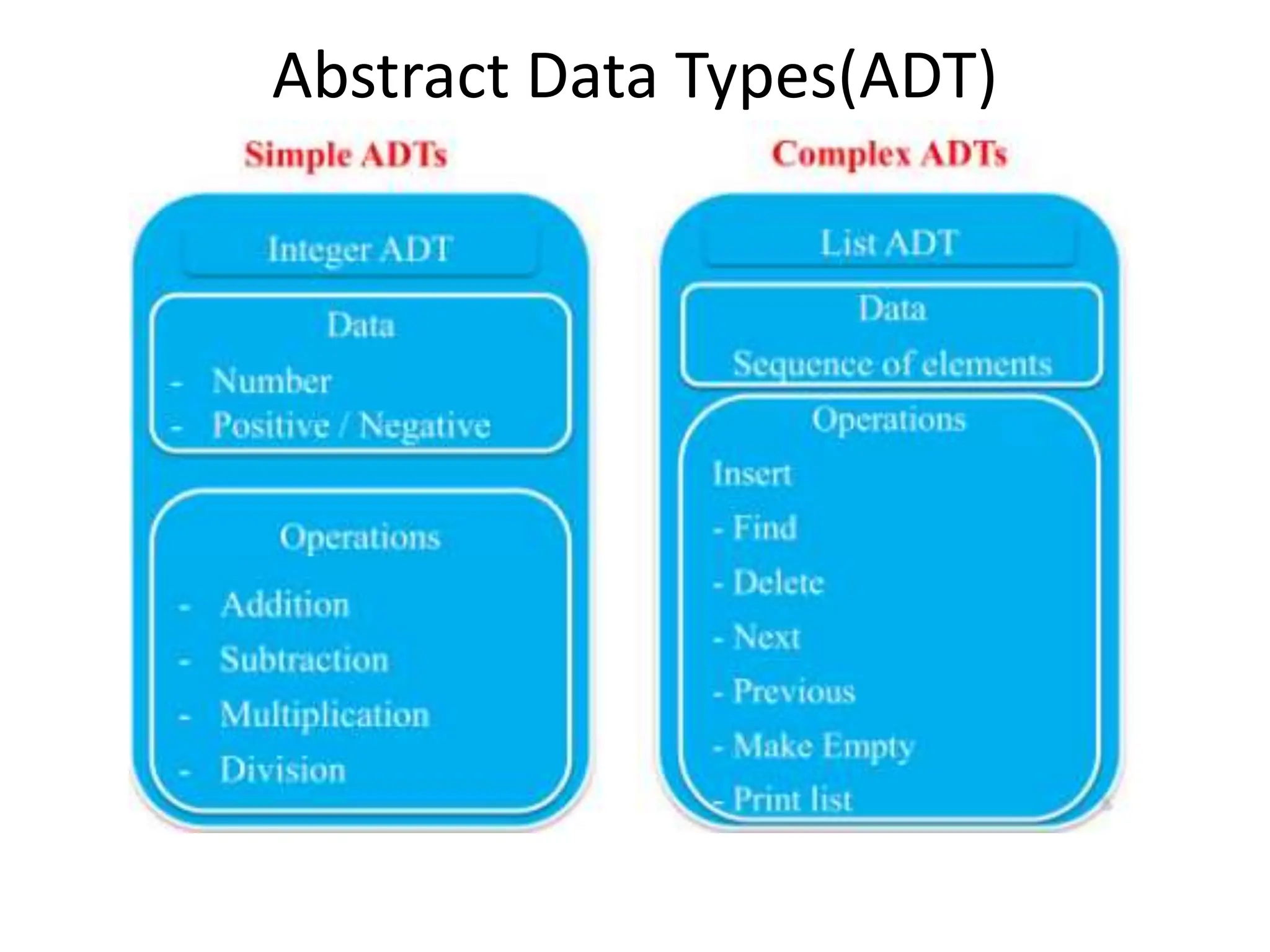
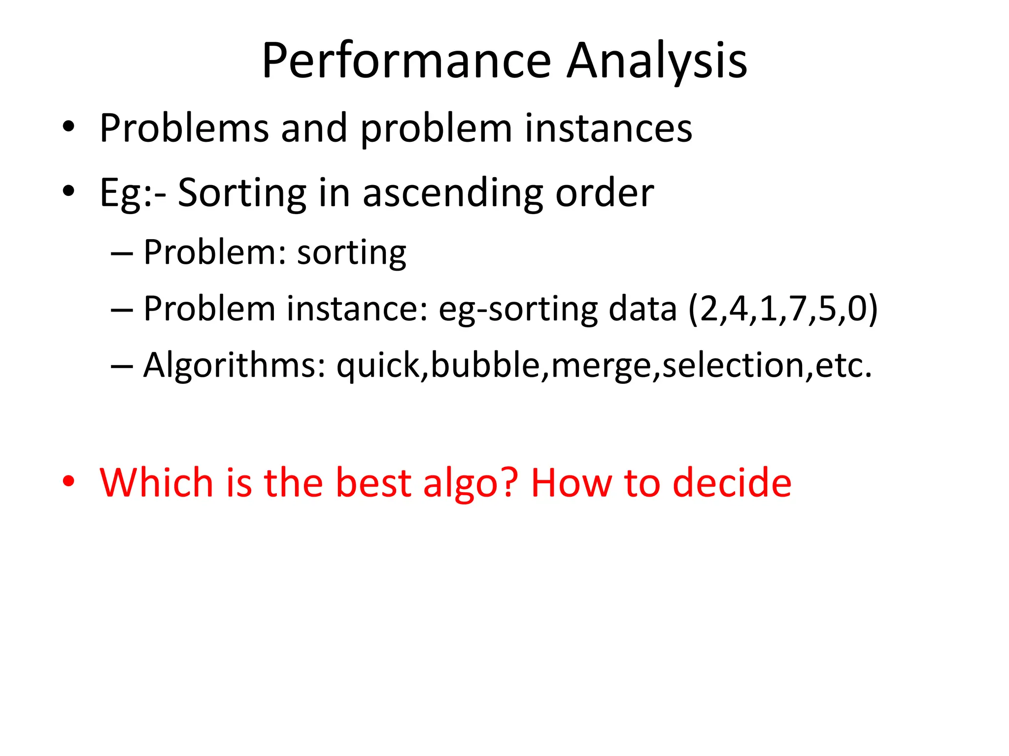
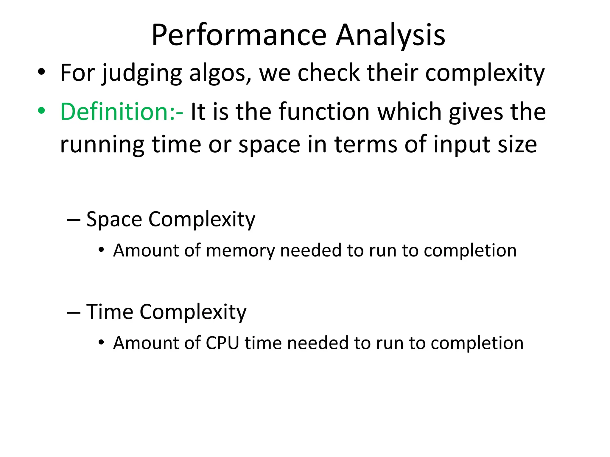
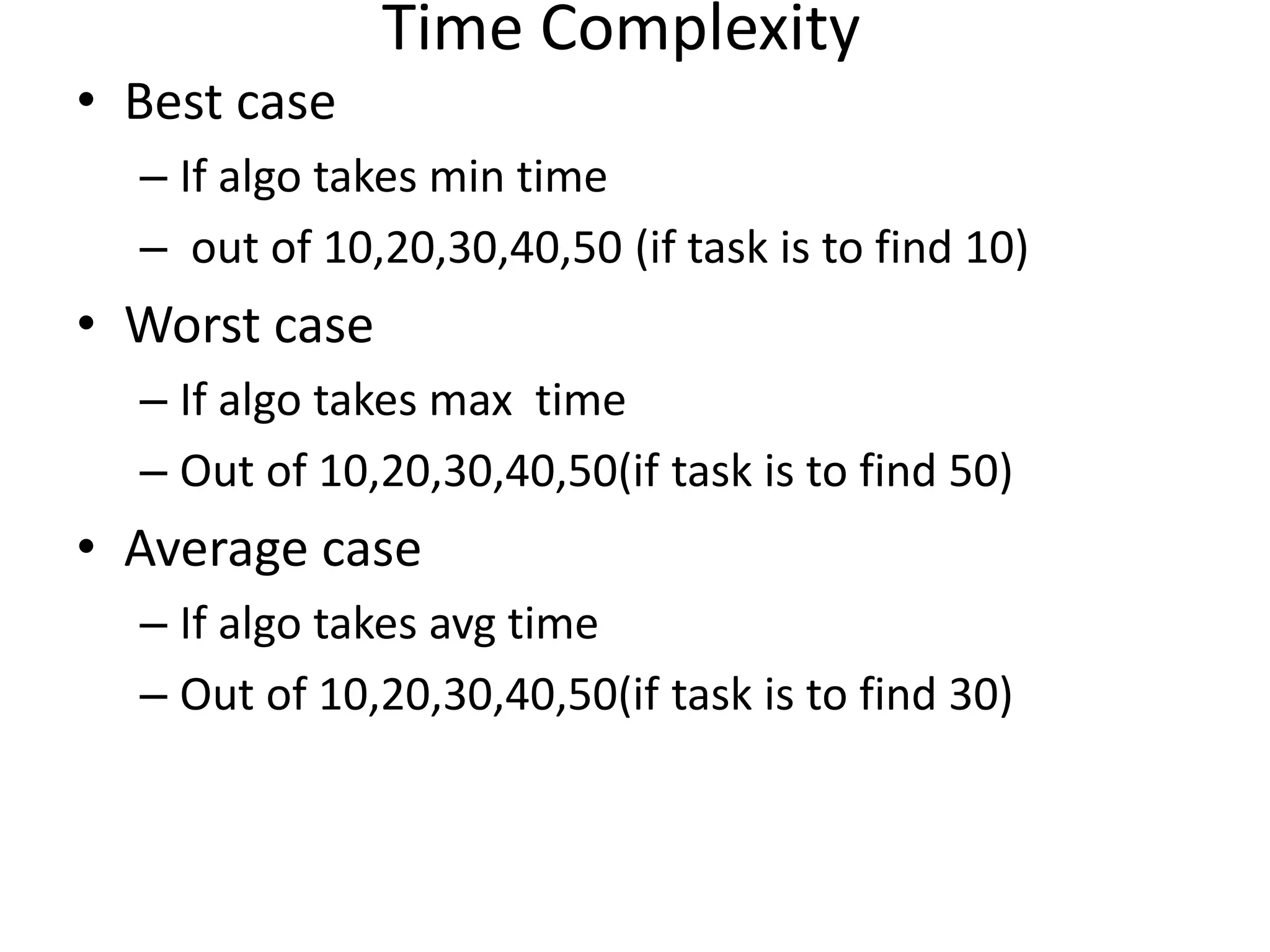
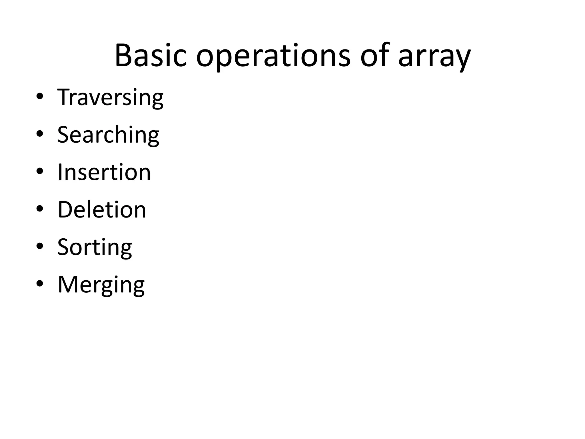
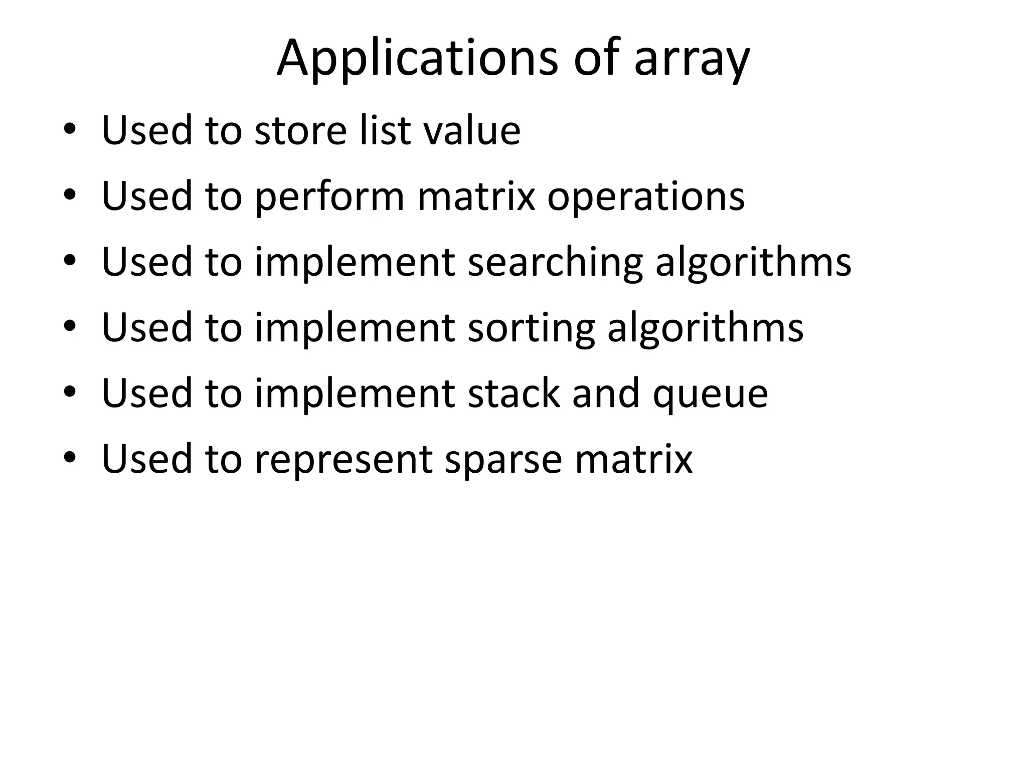
The document provides an introduction to data structures, classifying them into primitive and non-primitive types, and detailing operations and characteristics of each. It explains concepts related to abstract data types (ADT), performance analysis, and time and space complexity, along with methods for computing them. Additionally, it covers operations on arrays, such as traversing, inserting, and deleting elements, while also discussing two-dimensional arrays and their applications.
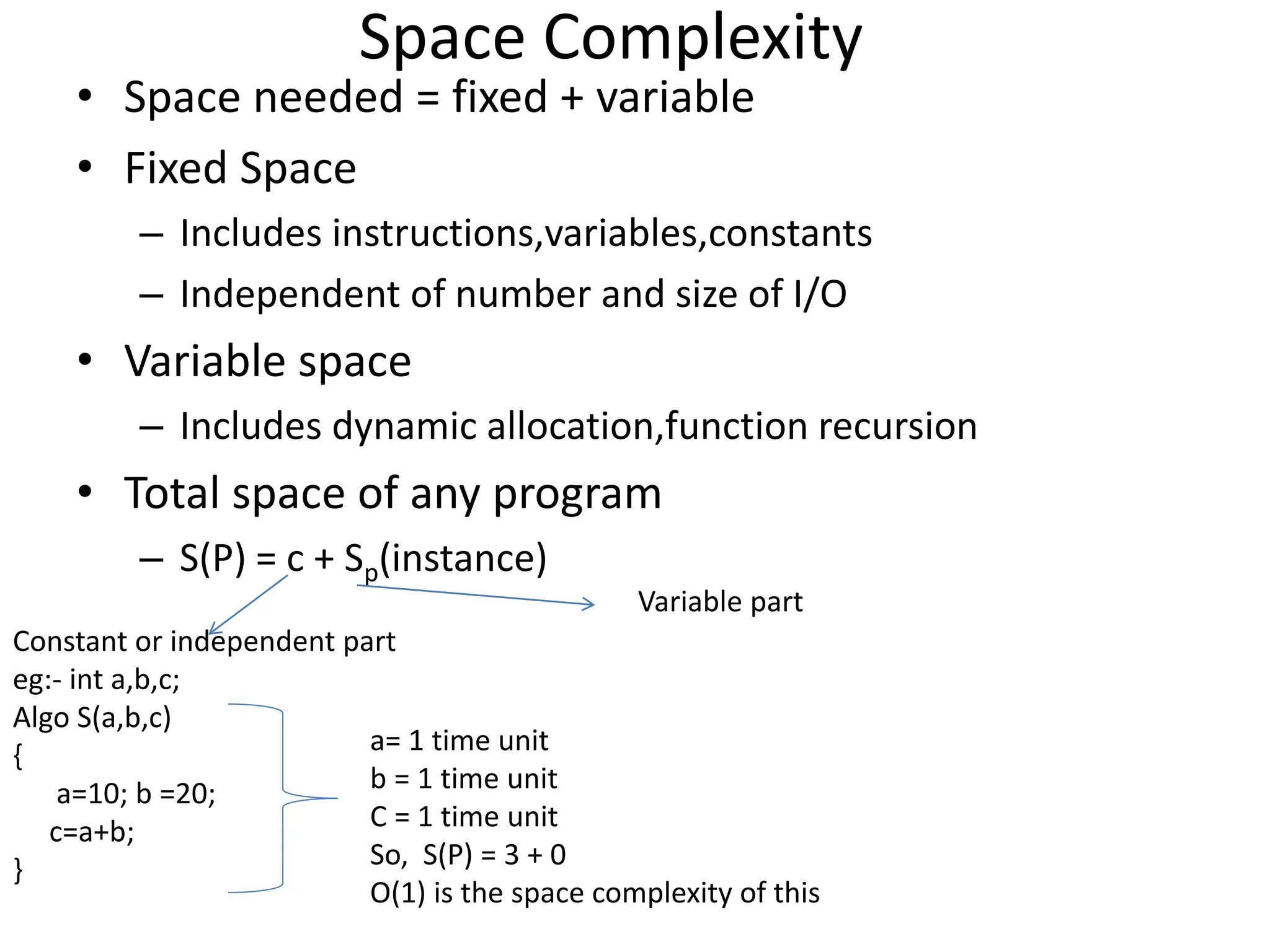
![Space Complexity • S(P) = c + Sp(instance) Variable part Eg:- let’s calculate sum of array a with n elements Algorithm Sum(a,n) { total =0; for i =0 to n do total = total + a[i]; } So , S(P) = c + Sp here , total , n and i are independent and so constant , so c =3. Now,calculating Sp . Here a is dependent on n. Suppose n=5, then size of a = 5*n S(P) = 3 + 5*n ignoring constants , O(n) is the complexity](https://image.slidesharecdn.com/unit-1-240504130735-059274e7/75/introduction-to-data-structures-and-types-16-2048.jpg)
![Time Complexity using frequency count • For comment and declaration – #program to add two arrays – Int a,b; – Step count = zero • For return and assignment – Int a=10; – return b; – Step count =1 • Ignore lower order exponent when higher order exponent are present – 3n4 + n3 + 5n2 + 23 = keep 3n4 , ignore the rest • Ignore constant multiplies – 3n4 ignore 3 from this • Sum (int a[],int n) { s=0; ------- 1 for(i=0;i<n;i++) -- n+1 (N TIMES CONDITION IS TRUE +1 FOR EXITING LOOP) s = s + a[i]; ---n return s; ---- 1 } So time complexity is 1+n+1+n+1 = 3+2n = O(n)](https://image.slidesharecdn.com/unit-1-240504130735-059274e7/75/introduction-to-data-structures-and-types-19-2048.jpg)
![Time complexity using asymptotic notation • Little Omega notation(ᵚ) – Let f(n),g(n) be two non-negative functions , then f(n)= ᵚ(g(n)) such that lim[g(n)/f(n)] = 0 , n- >infinity • Little Oh notation(o) – Let f(n),g(n) be two non-negative functions , then f(n)= o(g(n)) such that lim[f(n)/g(n)] = 0 , n->infinity](https://image.slidesharecdn.com/unit-1-240504130735-059274e7/75/introduction-to-data-structures-and-types-24-2048.jpg)
![Time Complexity-general rules Rule 1:- Loops Its running time = running time of statements in it. Eg:for(i=0;i<n;i++) -- n+1 times it runs { s = s +i; n times } So time complexity = n + n+1 = 2n+1 = O(n) Rule 2:- Nested Loops Its running time = total running time of statements inside a group of loops is the product of sizes of all loops Eg:- for(i=0;i<n;i++)--- n+1 { for(j=0; j<n;j++)---- n*(n+1) c[i][j]=a[i][j]+b[i][j];--n*n } So time complexity = n+n + n2+1 + n2 = 2n2 +2n + 1= O(n2) Rule 3:- consecutive statements Its running time = maximum one Eg- for(i=0;i<n;i++) --- n+1 s= s + i; -n for(i=0;i<n;i++) ---n+1 { for (j=0;j<n;j++) --n*(n+1) { c[i][j]=a[i][j]+b[i][j]; --- n*n } } So time complexity = 2n2+4n+2 = O(n2) Rule 4:- if-else Its running time = max of if or else Eg:- if (n<=0) --- 1 return n; ---- 1 else ---1 { for(i=0;i<n;i++) ----- n+1 s = s+ i; --n return s; --1 } so time complexity = 5 +2n = O(n)](https://image.slidesharecdn.com/unit-1-240504130735-059274e7/75/introduction-to-data-structures-and-types-25-2048.jpg)
![Data Structures: Arrays • Set of finite number of same data items • One dimensional array – An array with only one row or column – Elements are stored in continuous locations – Syntax is Datatype Array_name[size] – int abc[6] • 23 45 67 9 12 88 Maximum number of elements that can be stored in abc array 0 1 2 3 4 5 indexing Upper bound Lower bound 100 102 104 106 108 110 Base address Represe ntation of linear array in memory](https://image.slidesharecdn.com/unit-1-240504130735-059274e7/75/introduction-to-data-structures-and-types-27-2048.jpg)
![Data Structures: Arrays • Length/size of an array is given by following equation – (Upperbound -lowerbound) + 1 – For int abc[6] , it would be • (5-0) + 1 =6 • Array can be written or read through a loop – For(i=0;i<6;i++) { Scanf(“%d”,&abc[i]); Printf(“%d”,abc[i]); }](https://image.slidesharecdn.com/unit-1-240504130735-059274e7/75/introduction-to-data-structures-and-types-28-2048.jpg)
![Traversing arrays • Traversing:- used to access each element of array • Start from beginning and go till end of array and access value of each element exactly once • Eg:- int abc = {12,16,5,55,27} • Algorithm : Traversal(abc,LB,UB) abc is an array with lower bound LB and upper bound UB • Step 1: for LOC= LB to UB do • Step 2: Process abc[LOC] [End of for loop] • Step 3: exit](https://image.slidesharecdn.com/unit-1-240504130735-059274e7/75/introduction-to-data-structures-and-types-31-2048.jpg)
![Insertion into an array • Insertion at end • Algorithm – Let A be an array of size N – Step 1. If UB == N-1 • Then print overflow and exit – Step 2. Read data – Step 3. UB = UB+1 – Step 4. A[UB] =data – Step 5. Exit 3 2 6 8 0 1 2 3 4 UB 12](https://image.slidesharecdn.com/unit-1-240504130735-059274e7/75/introduction-to-data-structures-and-types-33-2048.jpg)
![Insertion into an array • Insertion at beginning • Algorithm – Let A be an array of size N – Step 1. If UB == N-1 • Then print overflow and exit – Step 2. Read data – Step 3. K=UB – Step 4. Repeat step 5 while K >= UB – Step 5. A[K+1]= A[K] K = K-1 – Step 6. A[LB] = data – Step 7. Stop 3 2 6 8 0 1 2 3 4 UB 12 Start from here 12 3 2 6 8 A[4] = A[3] A[3]= A[2] A[2]= A[1] A[1]=A[0] A[0] = data](https://image.slidesharecdn.com/unit-1-240504130735-059274e7/75/introduction-to-data-structures-and-types-34-2048.jpg)
![Insertion into an array • Insertion at a location • Algorithm – Let A be an array of size N – Step 1. If UB == N-1 • Then print overflow and exit – Step 2. Read data 12 – Step 3. Read LOC (LOC = 2) – Step 4. K=UB (k =3) – Step 5. Repeat step 6 while K >= LOC (3>=2) – Step 6. A[K+1] = A[K] K = K-1 – Step 7. A[LOC] = data – Step 8. Stop 3 2 6 8 0 1 2 3 4 UB 12 3 2 12 6 8 A[4] = A[3] K= 2 A[3] = A[2] K = 1 A[2]=12](https://image.slidesharecdn.com/unit-1-240504130735-059274e7/75/introduction-to-data-structures-and-types-35-2048.jpg)
![Deletion from end of an array • Deletion from end of array • Algorithm – Let A be an array of size N – Step 1. If UB == NULL • Then print underflow and exit – Step 2. A[UB] = NULL – Step 3. UB = UB-1 – Step 4. Stop 3 2 6 8 0 1 2 3 4 UB 3 2 6 LB 1 0 2 UB](https://image.slidesharecdn.com/unit-1-240504130735-059274e7/75/introduction-to-data-structures-and-types-37-2048.jpg)
![Deletion from start of an array • Deletion from start of array • Algorithm – Let A be an array of size N – Step 1. If UB == 0 • Then print underflow and exit – Step 2. K=LB – Step 3. Repeat step 4, while K< UB – Step 4. A[K] = A[K+1] K = K+1 – Step 5. A[UB] = NULL UB = UB -1 Stop 3 2 6 8 0 1 2 3 4 UB 2 6 8 LB 1 0 2 UB Shifting](https://image.slidesharecdn.com/unit-1-240504130735-059274e7/75/introduction-to-data-structures-and-types-38-2048.jpg)
![Deletion of a particular element of an array • Deletion of a particular element • Algorithm – Let A be an array of size N – Step 1. If UB == 0 • Then print underflow and exit – Step 2. Read DATA – Step 3. K = LB – Step 4. Repeat step 5 while A[K] = DATA – Step 5. K = K+1 – Step 6. Repeat step 7 while K < UB – Step 7. A[K] = A[K+1] K = K + 1 Stop – Step 8. A[UB] = NULL UB = UB -1 STOP 3 2 6 8 0 1 2 3 4 UB 3 2 8 LB 1 0 2 UB Shifting 9 9 3 Finding element to delete in array](https://image.slidesharecdn.com/unit-1-240504130735-059274e7/75/introduction-to-data-structures-and-types-39-2048.jpg)
![• Let’s find location (k) of an element • For 1d array – Loc(A[k]) = Base(A) + w*k – w = words per memory cell – Base(A) = starting address of array in memory](https://image.slidesharecdn.com/unit-1-240504130735-059274e7/75/introduction-to-data-structures-and-types-41-2048.jpg)
![• Consider an array A is declared as array of integers with size 50 and it’s first element is stored at memory address 101. So find out the address of 5th element. Given (w = 4) • Solution: - Given w = 4 , Base(A)=101 , k=5 – Formula is Loc(A[k]) = Base(A) + w*k – Loc(A[5]) = 101 + 4*5 = 121](https://image.slidesharecdn.com/unit-1-240504130735-059274e7/75/introduction-to-data-structures-and-types-42-2048.jpg)
![• Consider an array A, which records the number of t.v. sold each year from 1975 to 2000. Suppose that Base(A) = 101 and w = 4. Find out location of value of year 1990. • Solution :- Given w =4 and B(A) =101 – Formula is Loc(A[k]) = Base(A) + w*k – Let’s find k • 1990 -1975 = 15 = k – Now – Loc (A[15]) = 101 + 4*15 =161](https://image.slidesharecdn.com/unit-1-240504130735-059274e7/75/introduction-to-data-structures-and-types-43-2048.jpg)
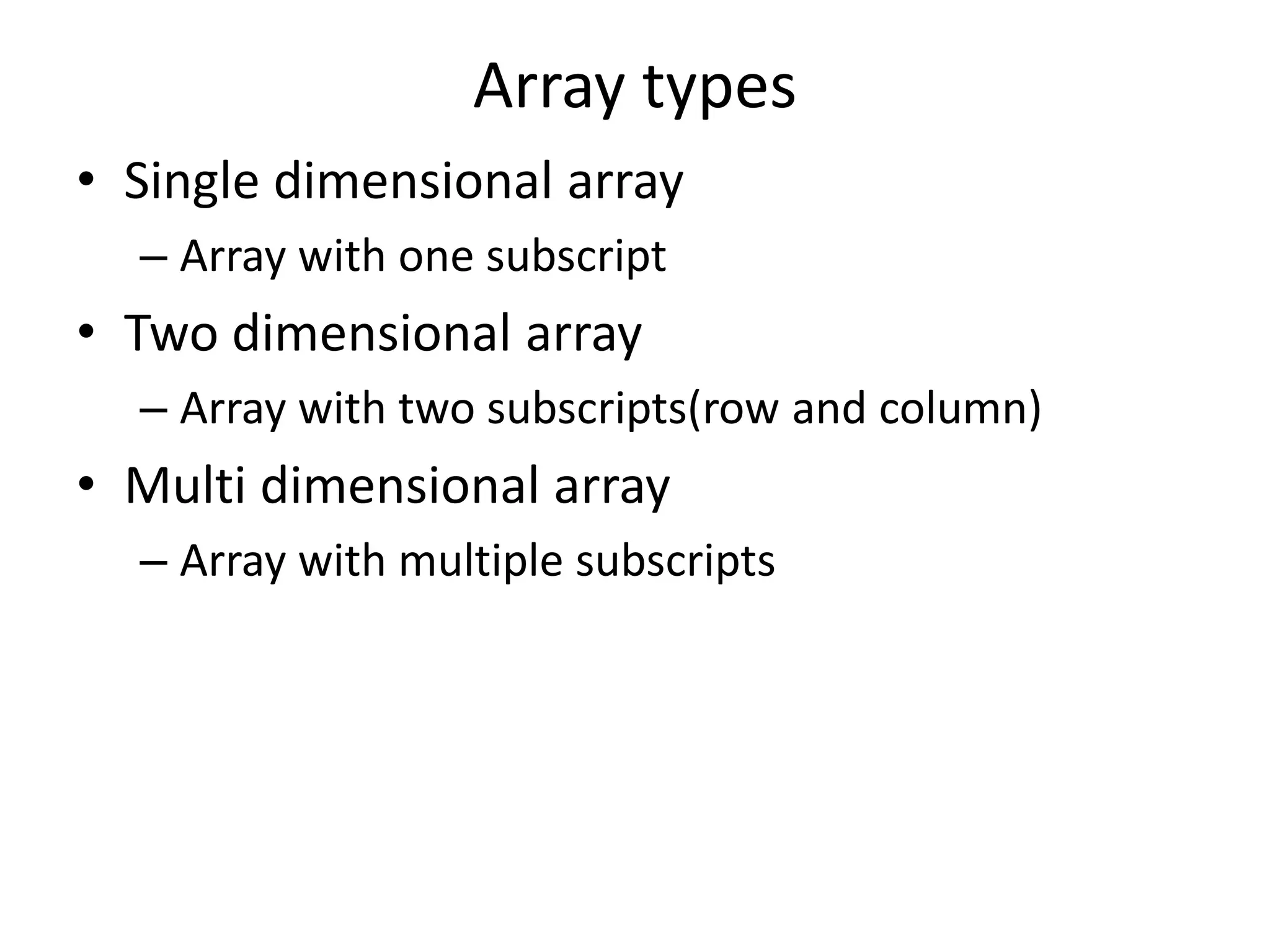
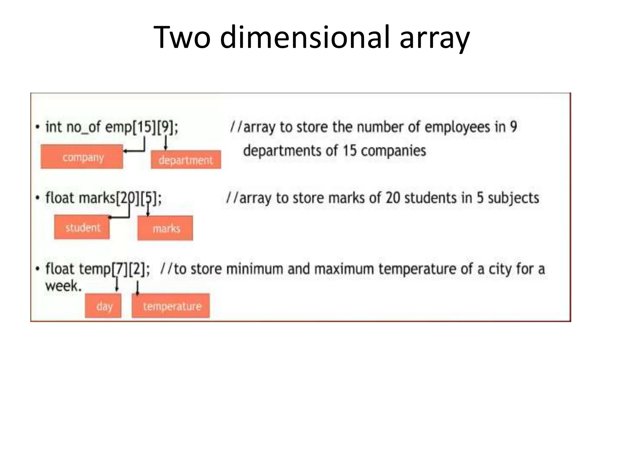
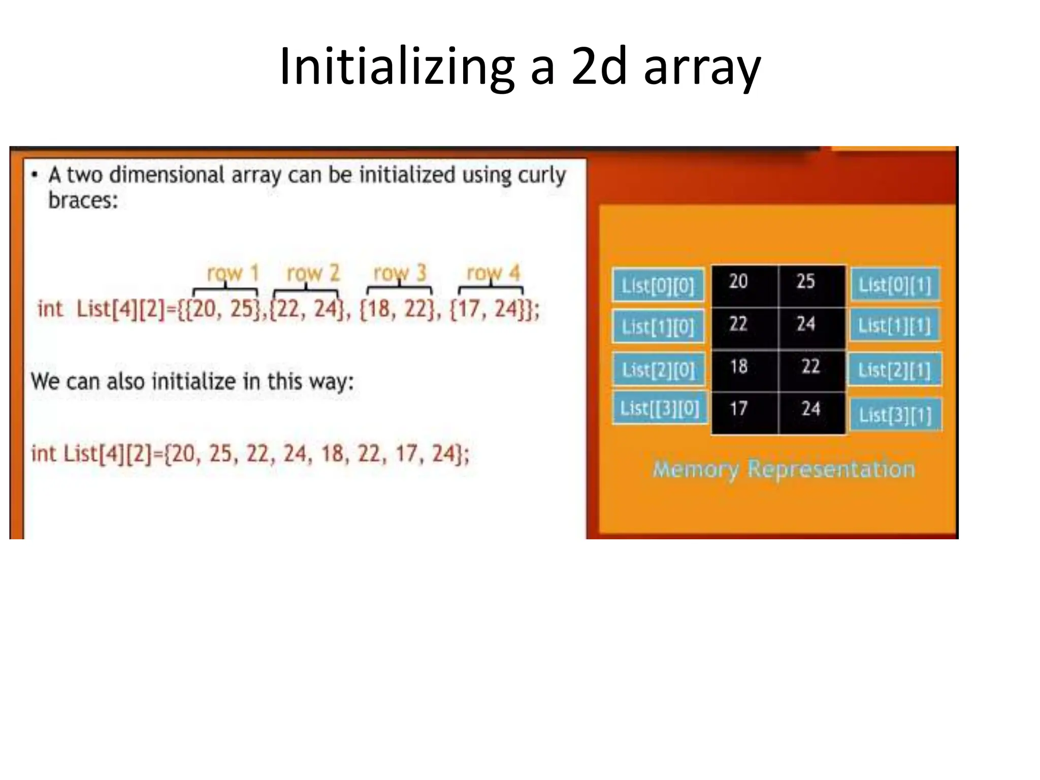
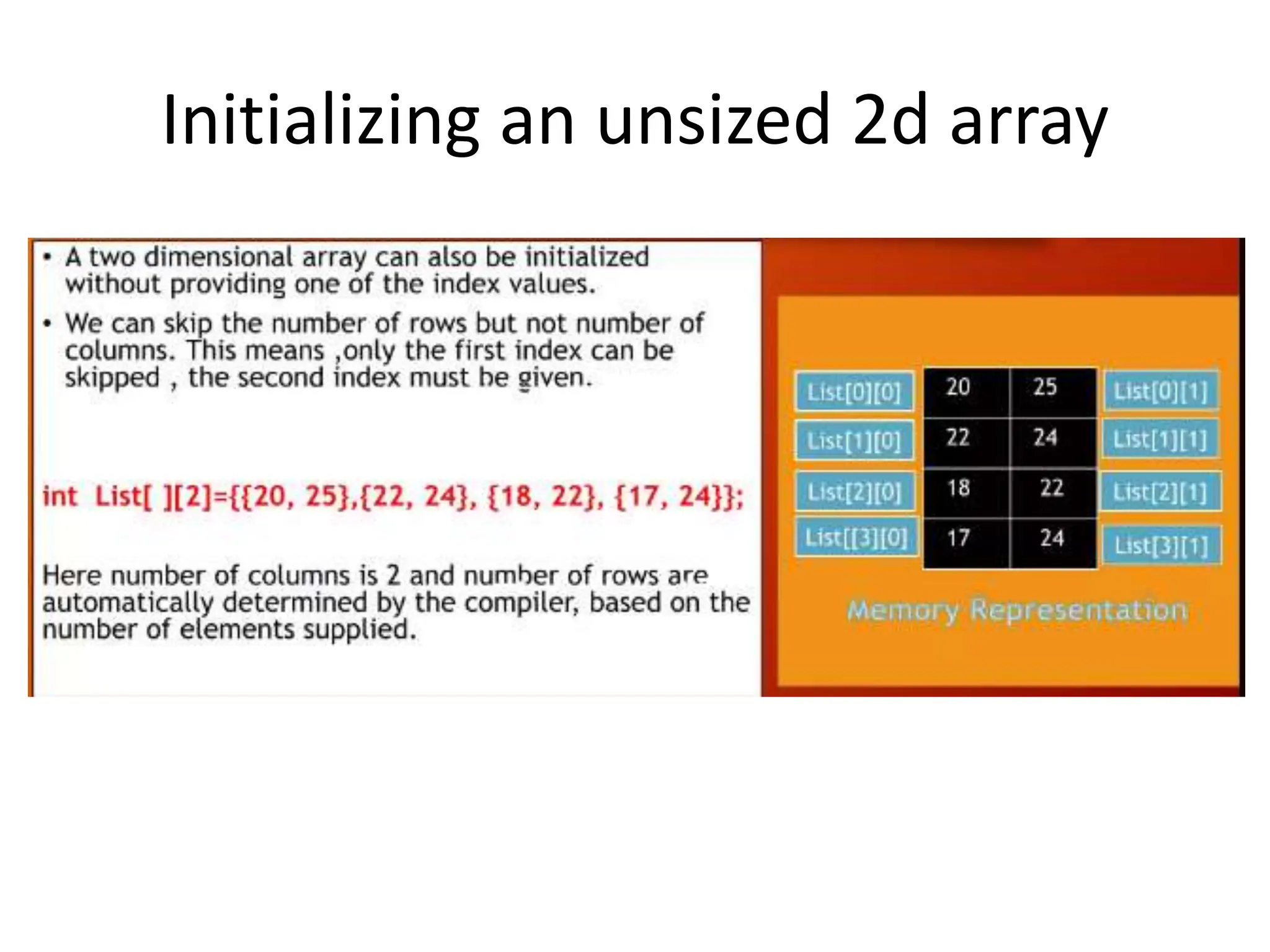
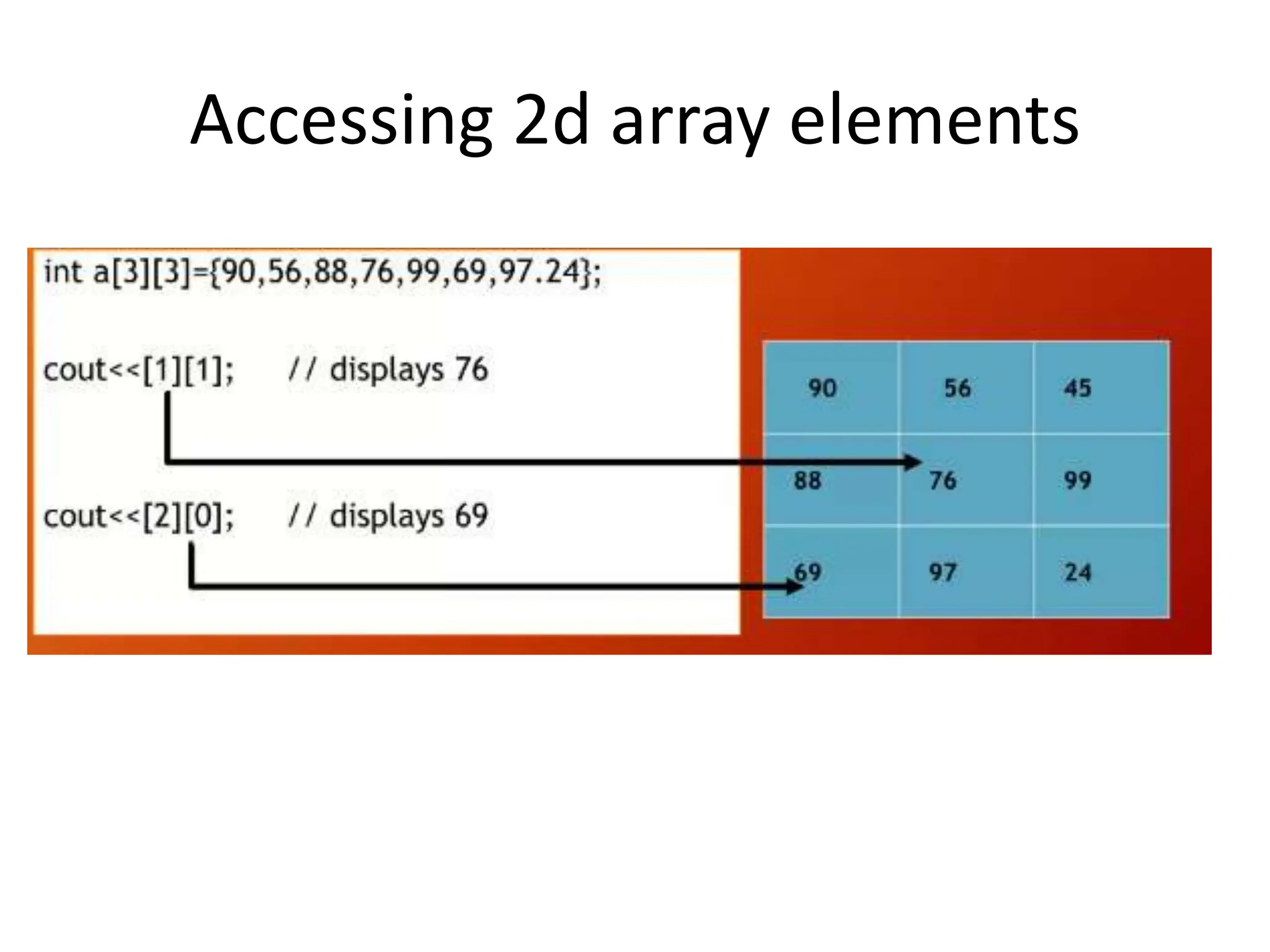
![Two dimensional array • Its arrangement of elements in rows and columns • Has two indices – 1st represents rows – 2nd represents columns • Eg:- int abc[4][4] • Datatype name[no of rows][no of columns]](https://image.slidesharecdn.com/unit-1-240504130735-059274e7/75/introduction-to-data-structures-and-types-45-2048.jpg)
![GTU Questions • Discuss various types of data structures with examples. [03] • Compare array and linked list[03] • Compare primitive and non primitive datatypes[04] • Differentiate between data types and data structures[03] • Answer the followings [04] – A) Give examples of linear and non linear data structures – B) What do you mean by abstract data types? • What is time complexity? Explain with example.[03] • Explain Asymptotic Notations in detail[07]](https://image.slidesharecdn.com/unit-1-240504130735-059274e7/75/introduction-to-data-structures-and-types-58-2048.jpg)