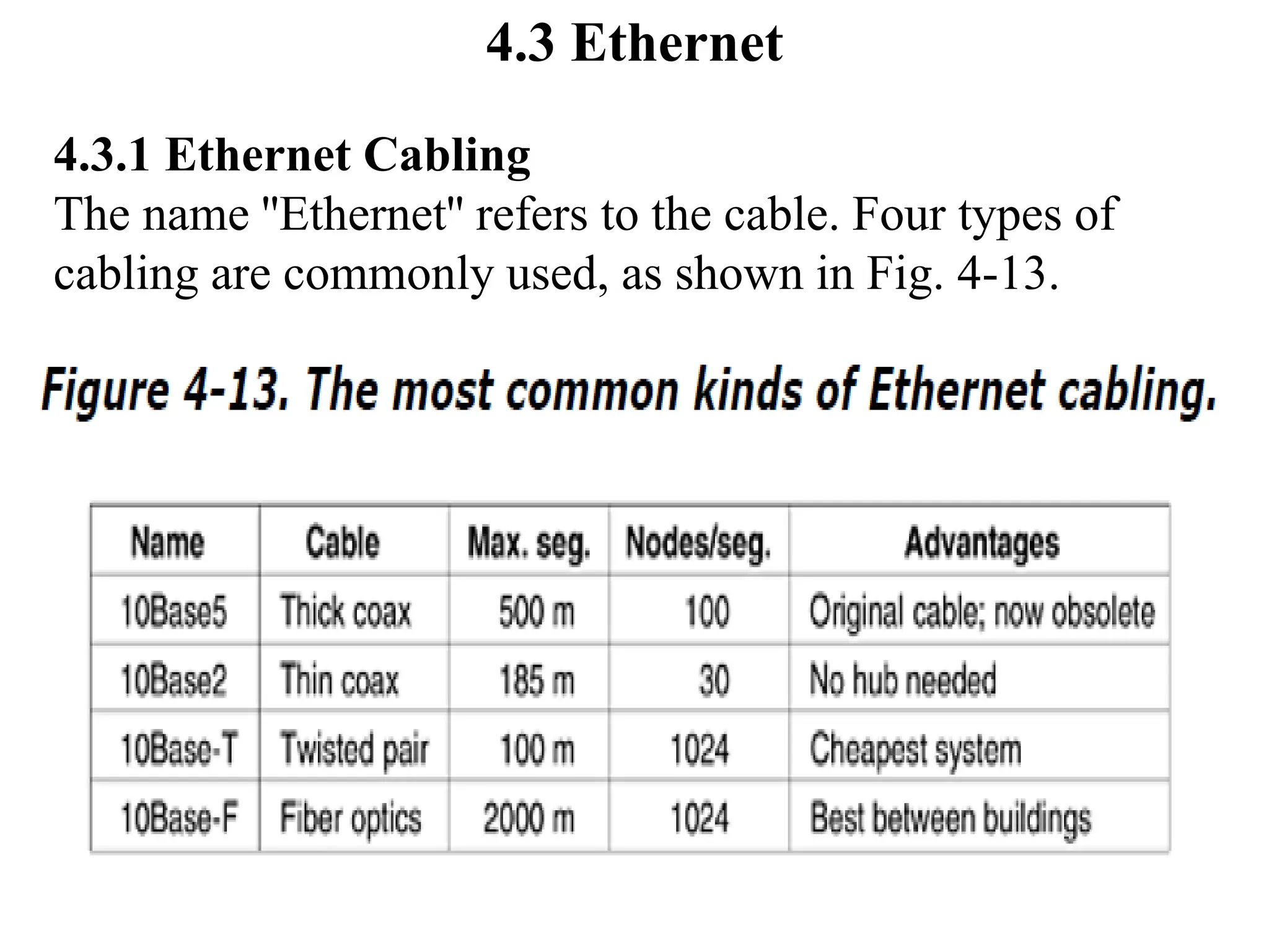
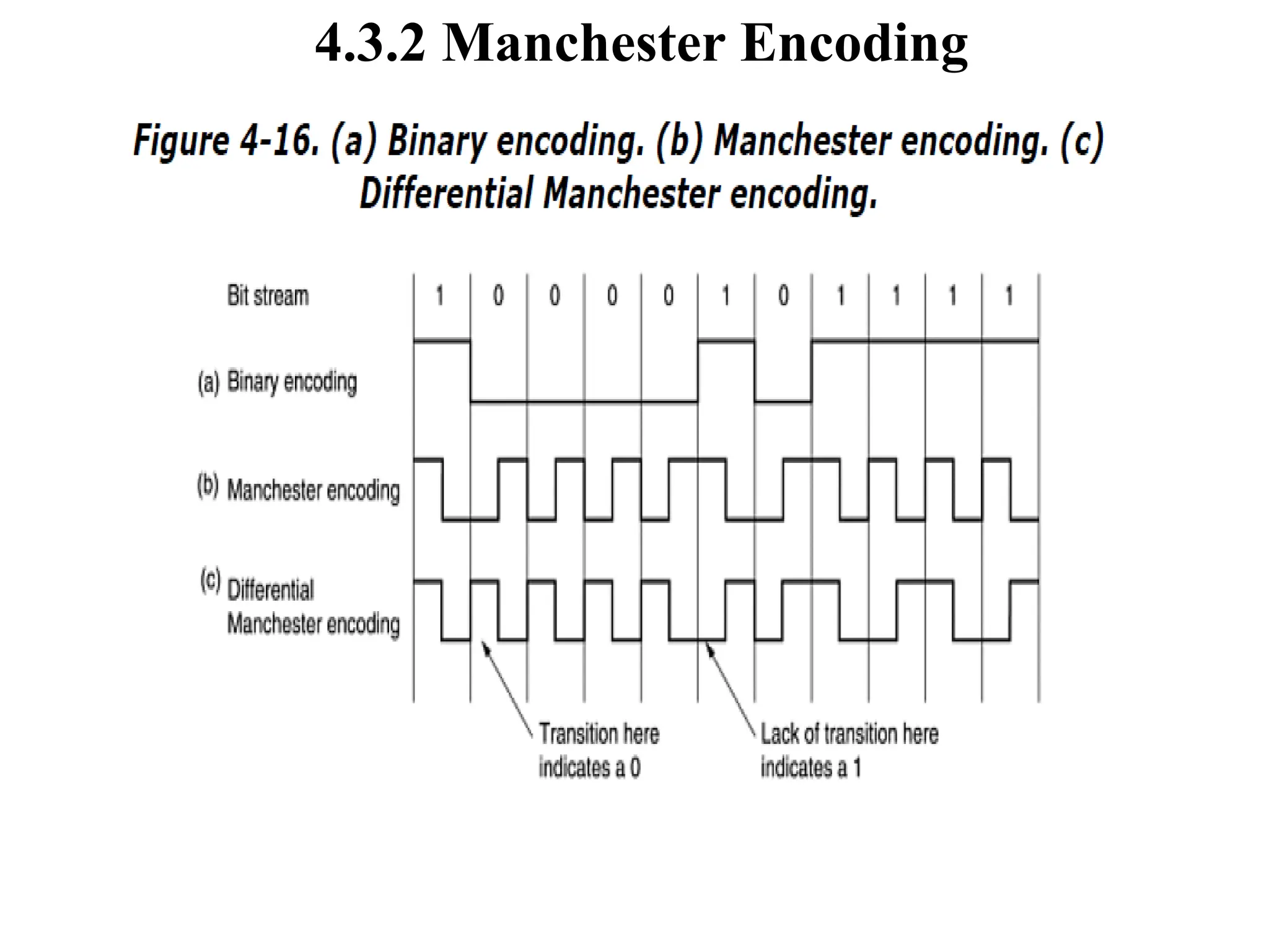
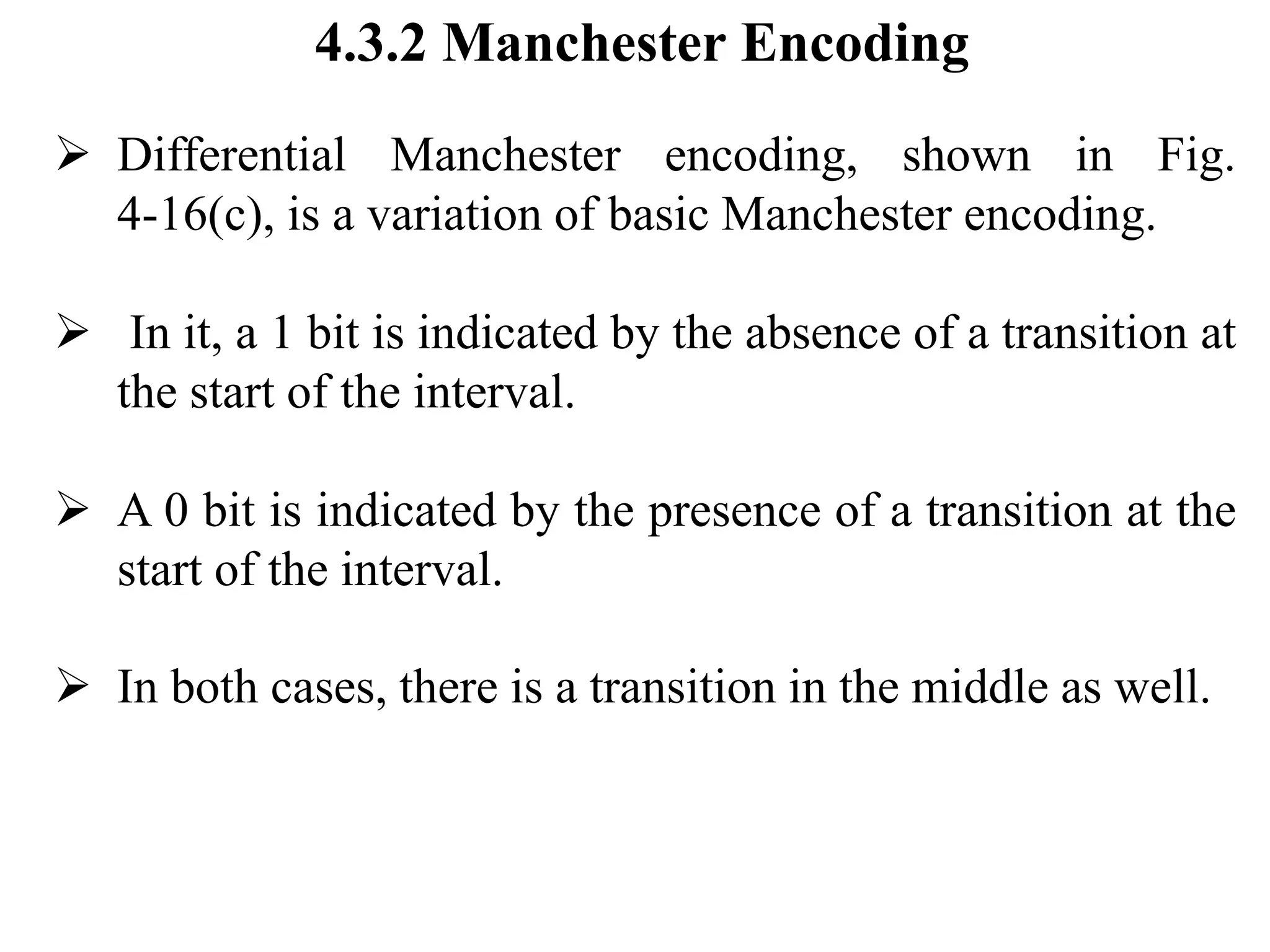
Lecture Notes Unit III PArt 2 - The DataLink Layer Medium Access Control Sublayer

Unit III- Part 2 - Data Link Layer - The Medium Access Control Sublayer Computer Network Dr. S.Murugan Associate Professor, Department of Computer Science. Alagappa Government Arts College, (Affiliated by Alagappa University) Karaikudi. Email: muruganjit@gmail.com

This slides compiled from Computer Network by Andrew S. Tenenbaum 4th Ed.

The Medium Access Control Sublayer ➢ In any broadcast network, the key issue is how to determine who gets to use the channel when there is competition for it. ➢ For example, consider a conference call in which six people, on six different telephones, are all connected so that each one can hear and talk to all the others. ➢ When one of them stops speaking, two or more will start talking at once, leading to collision. ➢ In a face-to-face meeting, chaos is avoided by external means, for example, at a meeting, people raise their hands to request permission to speak. The broadcast channels are sometimes referred to as multiaccess channels or random access channels.

The Medium Access Control Sublayer ➢ The protocols used to determine who goes next on a multiaccess channel belong to a sublayer of the data link layer called the MAC (Medium Access Control) sublayer. ➢ The MAC sublayer is especially important in LANs. ➢ MAC is responsible for the transmission of data packet to and from the network interface card. ➢ The Basic function of the MAC is to provide an addressing mechanism and channel access.

The Medium Access Control Sublayer ➢ so that each node available on the network can communicate with each other nodes available on the same or other network.

4.1 The Channel Allocation Problem ➢ The channel allocation problem deals with how to allocate a single broadcast channel among competing users.

4.1.1 Static Channel Allocation in LANs and MANs ➢ The traditional way of allocating a single channel, such as a telephone trunk, among multiple competing users is Frequency Division Multiplexing (FDM). ➢ If there are N users, the bandwidth is divided into N equal-sized portions and each user being assigned one portion. ➢ Since each user has a private frequency band, there is no interference between users.

4.1.1 Static Channel Allocation in LANs and MANs ➢ When the number of senders are large then the user may face the traffic problem. ➢ When there is only a small and constant number of users, each of which has a heavy (buffered) load of traffic (e.g., carriers' switching offices), FDM is a simple and efficient allocation mechanism

4.1.2 Dynamic Channel Allocation in LANs and MANs ➢ In dynamic channel allocation, would not fix any fixed number of users to each and every channel. The key assumption are as follows: ➢ 1. Station Model. The model consists of N independent stations (e.g., computers, telephones, or personal communicators), each with a program or user that generates frames for transmission. ➢ 2. Single Channel Assumption. A single channel is available for all communication. All stations can transmit on it and all can receive from it.

4.1.2 Dynamic Channel Allocation in LANs and MANs ➢ 3. Collision Assumption. If two frames are transmitted simultaneously, they overlap in time and the resulting signal is garbled. This event is called a collision. ➢ 4a. Continuous Time. Frame transmission can begin at any instant. (PURE ALOHA) ➢ 4b. Slotted Time. Time is divided into discrete intervals (slots). Frame transmissions always begin at the start of a slot. A slot may contain 0, 1, or more frames, corresponding to an idle slot, a successful transmission, or a collision, respectively. (SLOTTED ALOHA)

4.1.2 Dynamic Channel Allocation in LANs and MANs 5a. Carrier Sense. Before transmission, it checks whether the station is busy or not. If the channel is sensed as busy, no station will attempt to use it until it goes idle. 5b. No Carrier Sense. Before transmission, it did not check whether the station is busy or not. They just go ahead and transmit. Only later can they determine whether the transmission was successful.

4.2 Multiple Access Protocols ➢ In the 1970s, Norman Abramson and his colleagues initiated to develop a method to solve the channel allocation problem. ➢ ALOHA is a contention based protocol which means two or more nodes try to send messages across the network simultaneously. ➢ Two versions of ALOHA here: pure and slotted. They differ with respect to whether time is divided into discrete slots into which all frames must fit. ➢ Pure ALOHA does not require global time synchronization; slotted ALOHA does

4.2.1. ALOHA - Pure ALOHA ➢ The basic idea of an ALOHA system is simple: let users transmit whenever they have data to be sent. ➢ There will be collisions, of course, and the colliding frames will be damaged. ➢ If the frame was destroyed, the sender just waits a random amount of time and sends it again. ➢ The waiting time must be random or the same frames will collide over and over, in lockstep. ➢ Systems in which multiple users share a common channel in a way that can lead to conflicts are widely known as contention systems.

➢ A sketch of frame generation in an ALOHA system is given in Fig. 4-1. 4.2.1. ALOHA - Pure ALOHA

➢ All the frames are the same length. ➢ Whenever two frames, try to occupy the channel at the same time, there will be a collision and both will be garbled. ➢ If the first bit of a new frame overlaps with just the last bit of a frame almost finished, both frames will be totally destroyed and both will have to be retransmitted later. 4.2.1. ALOHA - Pure ALOHA

ALOHA - Slotted ALOHA ➢ In 1972, Roberts published a method for doubling the capacity of an ALOHA system known as slotted aloha. ➢ In slotted aloha, time is divided into particular slots. ➢ Every node can transmit the data only at the beginning of the slot. ➢ A sketch of frame generation in an ALOHA system is given as follows.

ALOHA - Slotted ALOHA ➢ Node A transmits the data at time t1 and Node B transmits the data at time t2. ➢ If the node C wants to transmit the data at time t3, the node c has to wait until the node B complete its transmission. ➢ If Node A and Node C transmit the data simultaneously, then collision will occur.

Difference between Pure ALOHA and Slotted ALOHA S. No Pure Aloha Slotted Aloha 1. A Node can transmit data at any time A Node can transmit the data at the particular time slot. If a node misses the slot, it has to wait until the beginning of the next slot. 2. Divide the time into the continuous interval Divide the time into the discrete interval 3. Developed by Norman Abramson in 1970. Developed by Roberts in 1972. 4. Channel utilization is 18% Channel utilization is 36%

4.2.2 Carrier Sense Multiple Access Protocols ➢ Protocols, in which stations listen for a carrier (i.e., a transmission) and act accordingly are called carrier sense protocols. Persistent CSMA ➢ The station continuously sensing until the channel is idle. non-Persistent CSMA ➢ The station wait for a random period of time. P-persistent ➢ The station will wait for a next time slot instead of random period of time. CSMA with CD ➢ The station abort its transmission, if the collision detects.

4.2.2 Carrier Sense Multiple Access Protocols ➢ Protocols, in which stations listen for a carrier (i.e., a transmission) and act accordingly are called carrier sense protocols. Persistent CSMA ➢ The first carrier sense protocol is called 1-persistent CSMA (Carrier Sense Multiple Access). ➢ When a station has data to send, it first listens to the channel to see if anyone else is transmitting at that moment. ➢ If the channel is busy, the station waits until it becomes idle.

4.2.2 Carrier Sense Multiple Access Protocols ➢ When the station detects an idle channel, it transmits a frame. ➢ If a collision occurs, the station waits a random amount of time and starts all over again. ➢ The protocol is called 1-persistent because the station transmits with a probability of 1 when it finds the channel idle.

4.2.2 Carrier Sense Multiple Access Protocols Nonpersistent CSMA ➢ A second carrier sense protocol is nonpersistent CSMA. ➢ In this protocol, Before sending, a station senses the channel. ➢ If no one else is sending, the station begins doing so itself. ➢ However, if the channel is already in use, the station does not continually sense it for the purpose of seizing it immediately upon detecting the end of the previous transmission.

4.2.2 Carrier Sense Multiple Access Protocols Nonpersistent CSMA ➢ Instead, it waits a random period of time and then repeats the algorithm. ➢ Consequently, this algorithm leads to better channel utilization but longer delays than 1-persistent CSMA.

4.2.2 Carrier Sense Multiple Access Protocols ➢ The last protocol is p-persistent CSMA. It applies to slotted channels and works as follows. ➢ When a station becomes ready to send, it senses the channel. ➢ If it is idle, it transmits with a probability p. With a probability q = 1 - p, it defers until the next slot. ➢ If that slot is also idle, it either transmits or defers again, with probabilities p and q. ➢ This process is repeated until either the frame has been transmitted or another station has begun transmitting.

4.2.2 Carrier Sense Multiple Access Protocols ➢ Persistent and nonpersistent CSMA protocols are clearly an improvement over ALOHA because they ensure that no station begins to transmit when it senses the channel busy. ➢ CSMA/CD (CSMA with Collision Detection) Another improvement is for stations to abort their transmissions as soon as they detect a collision. ➢ In other words, if two stations sense the channel to be idle and begin transmitting simultaneously, they will both detect the collision almost immediately.

4.2.2 Carrier Sense Multiple Access Protocols ➢ Rather than finish transmitting their frames, which are irretrievably garbled anyway, they should abruptly stop transmitting as soon as the collision is detected. ➢ Quickly terminating damaged frames saves time and bandwidth. ➢ This protocol, known as CSMA/CD (CSMA with Collision Detection) is widely used on LANs in the MAC sublayer.

4.3.1 Ethernet Cabling The name ''Ethernet'' refers to the cable. Four types of cabling are commonly used, as shown in Fig. 4-13. 4.3 Ethernet

➢ 10Base5 cabling, popularly called thick Ethernet, came first. ➢ It resembles a yellow garden hose. ➢ The notation 10Base5 means that it operates at 10 Mbps, uses baseband signaling, and can support segments of up to 500 meters. ➢ The first number is the speed in Mbps. Then comes the word ''Base'' (or sometimes ''BASE'') to indicate baseband transmission. 4.3 Ethernet

➢ The second cable type was 10Base2, or thin Ethernet, which, in contrast to the ➢ garden-hose-like thick Ethernet, bends easily. ➢ Thin Ethernet is much cheaper and easier to install, but it can run for only 185 meters per segment, each of which can handle only 30 machines. 4.3 Ethernet

➢ The third cable type was 10Base-T, or Twisted pair. ➢ All stations have a cable running to a central hub in which they are all connected electrically. ➢ Usually, these wires are telephone company twisted pairs. This scheme is called 10Base-T. ➢ 4.3 Ethernet

➢ A fourth cabling option for Ethernet is 10Base-F, which uses fiber optics. ➢ This alternative is expensive due to the cost of the connectors and terminators, but it has excellent noise immunity and is the method of choice when running between buildings or widely-separated hubs. ➢ Runs of up to km are allowed. 4.3 Ethernet

➢ Figure 4-15 shows different ways of wiring a building. ➢ In Fig. 4-15(a), a single cable is snaked from room to room, with each station tapping into it at the nearest point. ➢ In Fig. 4-15(b), a vertical spine runs from the basement to the roof, with horizontal cables on each floor connected to the spine by special amplifiers (repeaters). In some buildings, the horizontal cables are thin and the backbone is thick. 4.3.2 Cable Topologies

➢ The most general topology is the tree, as in Fig. 4- 15(c), because a network with two paths between some pairs of stations would suffer from interference between the two signals. ➢ Each version of Ethernet has a maximum cable length per segment. ➢ To allow larger networks, multiple cables can be connected by repeaters, as shown in Fig. 4-15(d). ➢ A repeater is a physical layer device. It receives, amplifies (regenerates), and retransmits signals in both directions. 4.3 Ethernet - Cable Topologies

4.3 Ethernet - Cable Topologies

➢ None of the versions of Ethernet uses straight binary encoding with 0 volts for a 0 bit and 5 volts for a 1 bit. ➢ This problem can be solved by using +1 volts for a 1 and -1 volts for a 0. ➢ ➢ With Manchester encoding, each bit period is divided into two equal intervals. ➢ A binary 1 bit is sent by having the voltage set high during the first interval and low in the second one. ➢ A binary 0 is just the reverse: first low and then high. 4.3.2 Manchester Encoding

➢ This scheme ensures that every bit period has a transition in the middle, making it easy for the receiver to synchronize with the sender. ➢ A disadvantage of Manchester encoding is that it requires twice as much bandwidth as straight binary encoding because the pulses are half the width. ➢ Manchester encoding is shown in Fig. 4-16(b). 4.3.2 Manchester Encoding

➢ Differential Manchester encoding, shown in Fig. 4-16(c), is a variation of basic Manchester encoding. ➢ In it, a 1 bit is indicated by the absence of a transition at the start of the interval. ➢ A 0 bit is indicated by the presence of a transition at the start of the interval. ➢ In both cases, there is a transition in the middle as well. 4.3.2 Manchester Encoding

Lecture Notes Unit III PArt 2 - The DataLink Layer Medium Access Control Sublayer

More Related Content

What's hot

Similar to Lecture Notes Unit III PArt 2 - The DataLink Layer Medium Access Control Sublayer

More from Murugan146644

Recently uploaded

Lecture Notes Unit III PArt 2 - The DataLink Layer Medium Access Control Sublayer