COMPUTER VISION (Module-2) Dr.Ramesh Wadawadagi Associate Professor Department of CSE SVIT, Bengaluru-560064 ramesh.sw@saividya.ac.in More neighborhood operators
2.
Non-linear filtering ● Inliear filtering each output pixel is estimated as a weighted sum of neighborhood input pixels. ● Linear filters are easier to compose and are compliant to frequency response analysis. ● In many cases, however, better performance can be obtained by using a non-linear combination of neighboring pixels. ● In this chapter, we will discuss some non-linear filters applied for image enhancement task.
3.
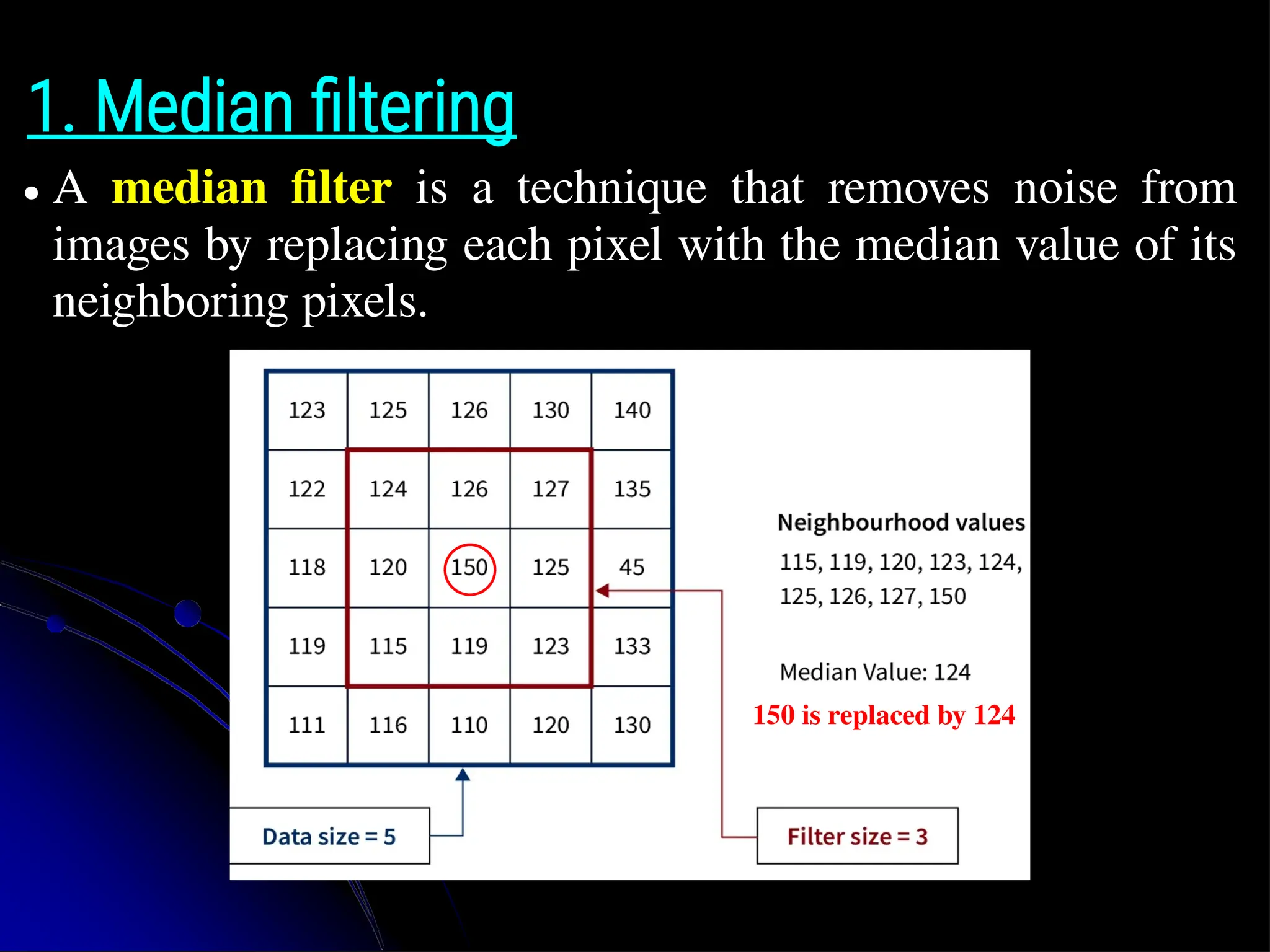
1. Median filtering ●A median filter is a technique that removes noise from images by replacing each pixel with the median value of its neighboring pixels. 150 is replaced by 124
4.
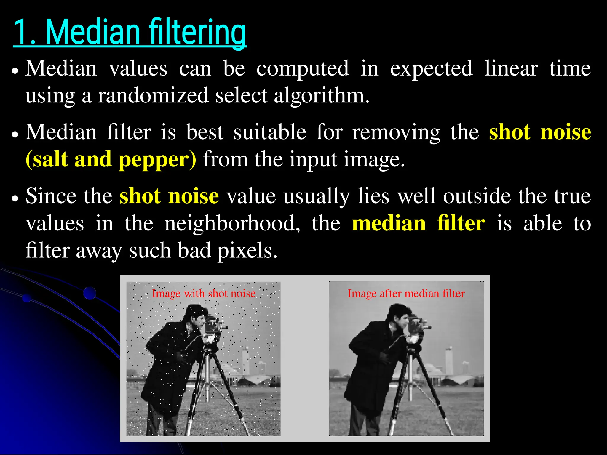
1. Median filtering ●Median values can be computed in expected linear time using a randomized select algorithm. ● Median filter is best suitable for removing the shot noise (salt and pepper) from the input image. ● Since the shot noise value usually lies well outside the true values in the neighborhood, the median filter is able to filter away such bad pixels. Image with shot noise Image after median filter
5.
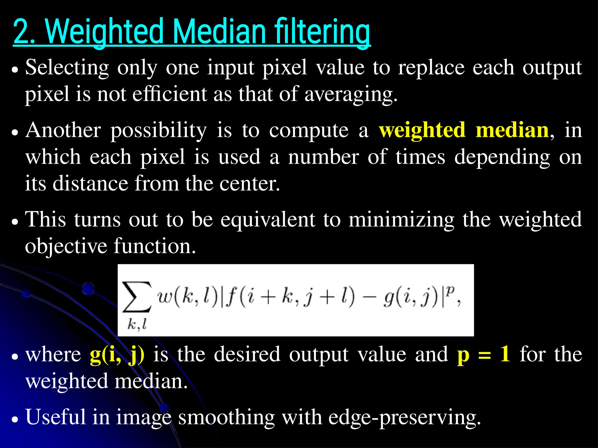
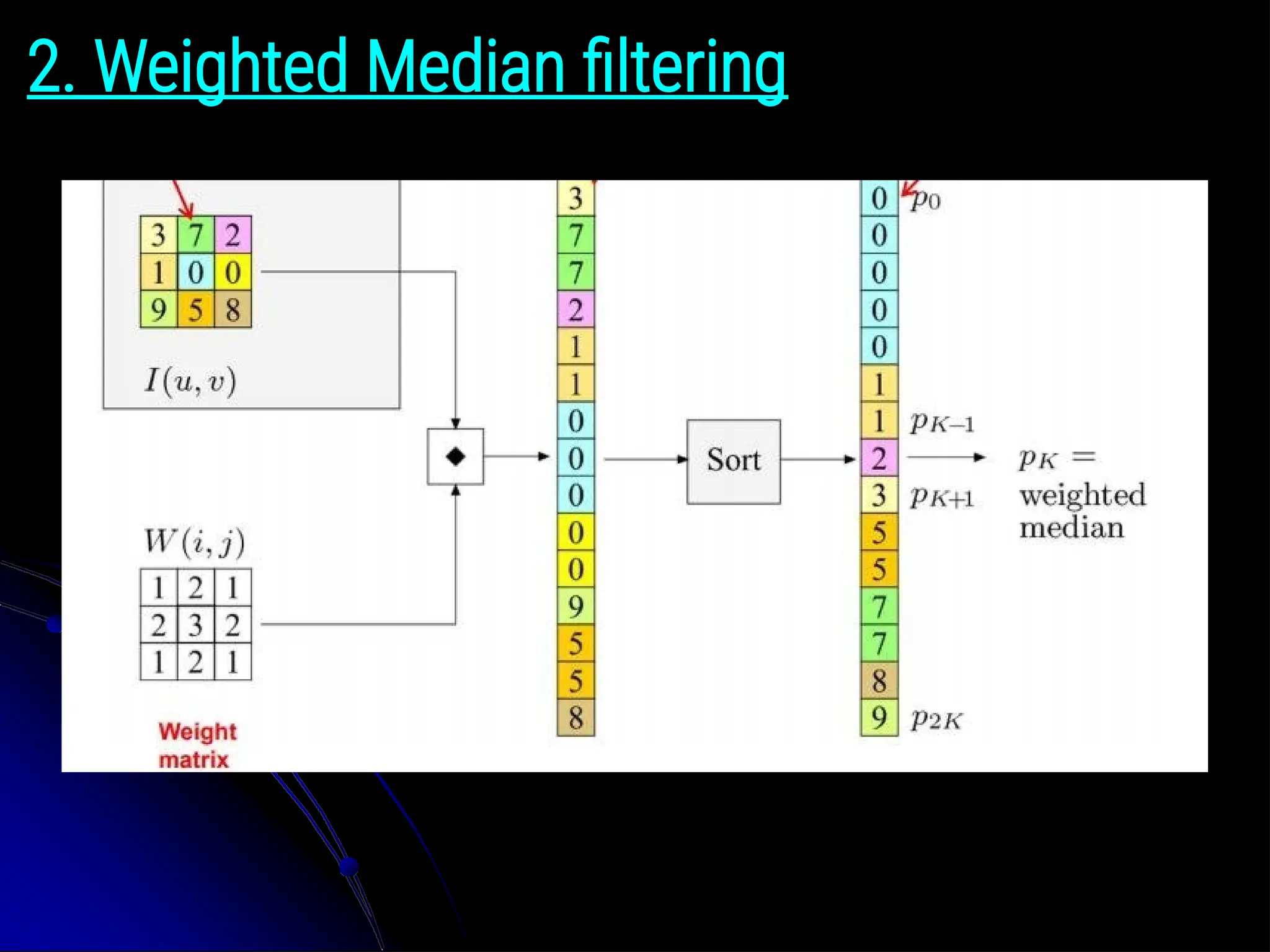
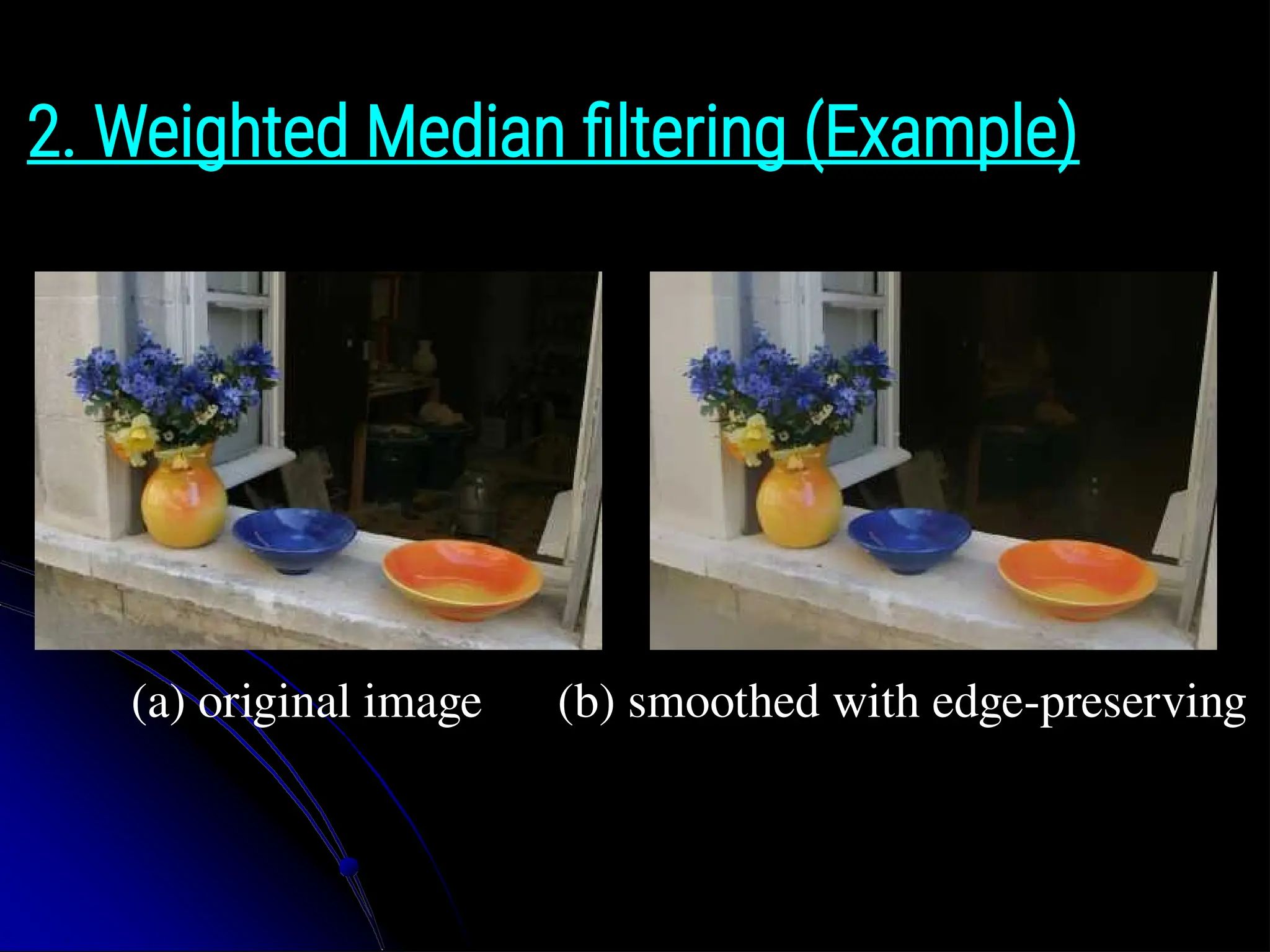
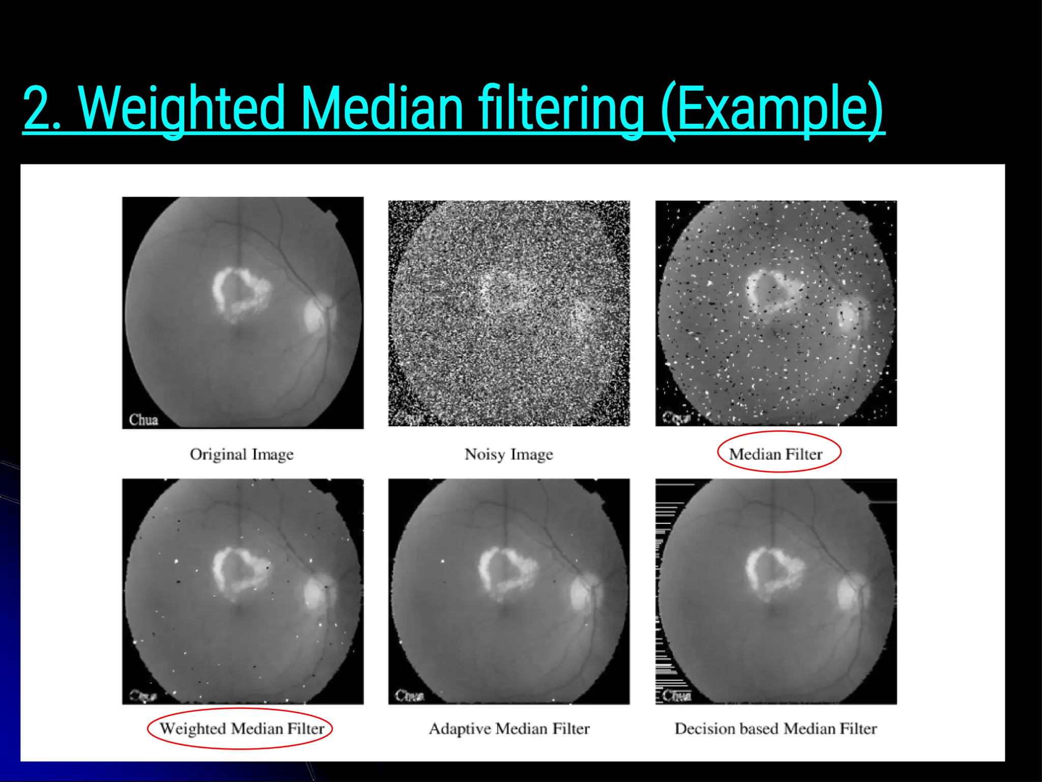
2. Weighted Medianfiltering ● Selecting only one input pixel value to replace each output pixel is not efficient as that of averaging. ● Another possibility is to compute a weighted median, in which each pixel is used a number of times depending on its distance from the center. ● This turns out to be equivalent to minimizing the weighted objective function. ● where g(i, j) is the desired output value and p = 1 for the weighted median. ● Useful in image smoothing with edge-preserving.
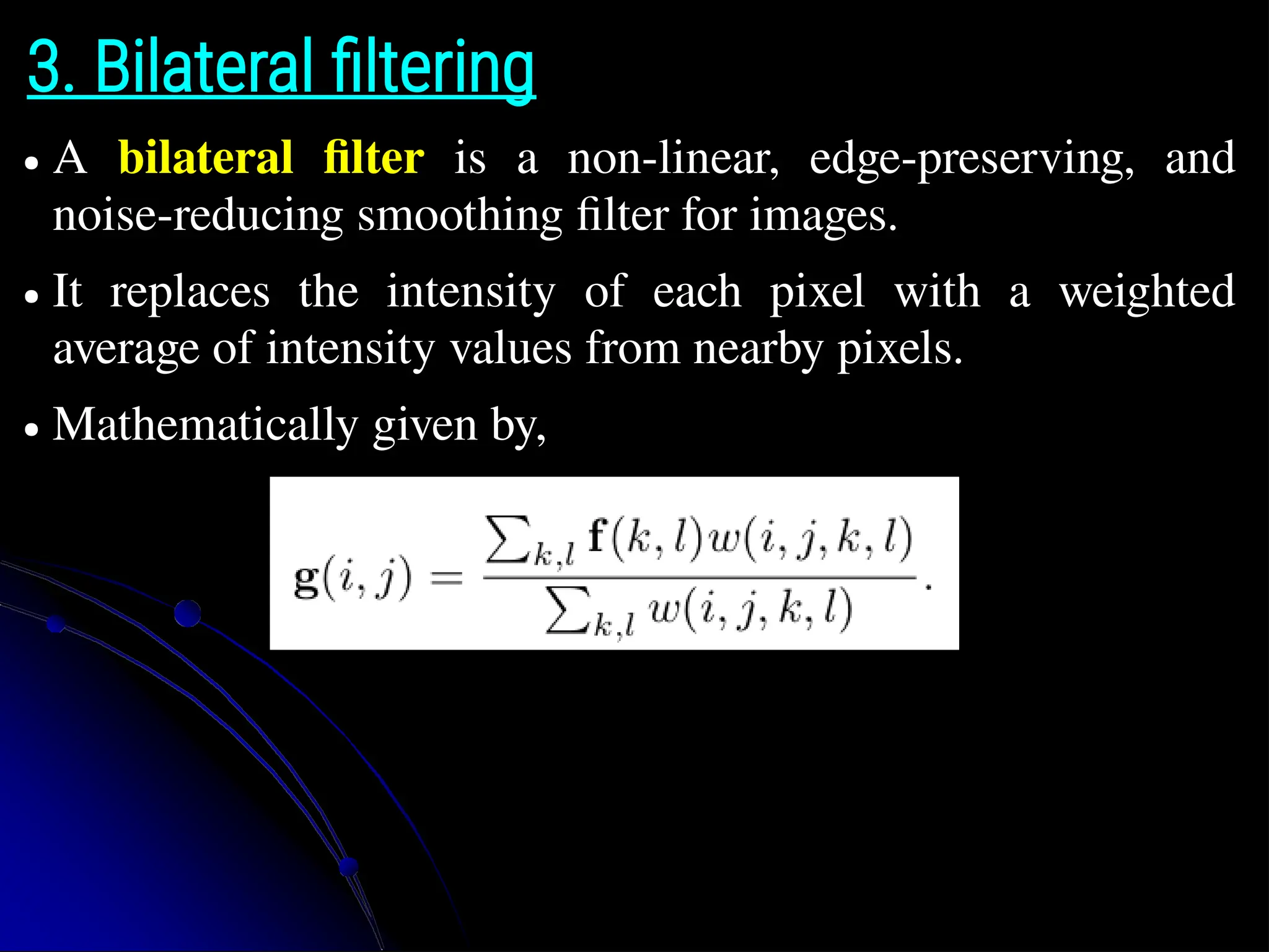
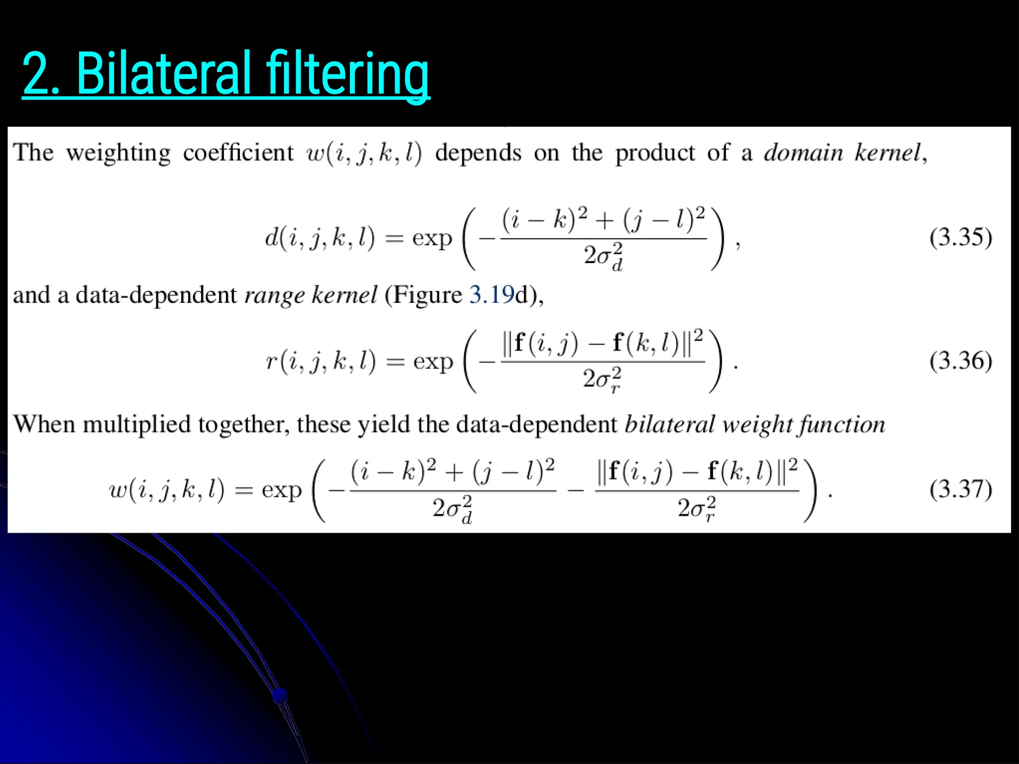
3. Bilateral filtering ●A bilateral filter is a non-linear, edge-preserving, and noise-reducing smoothing filter for images. ● It replaces the intensity of each pixel with a weighted average of intensity values from nearby pixels. ● Mathematically given by,
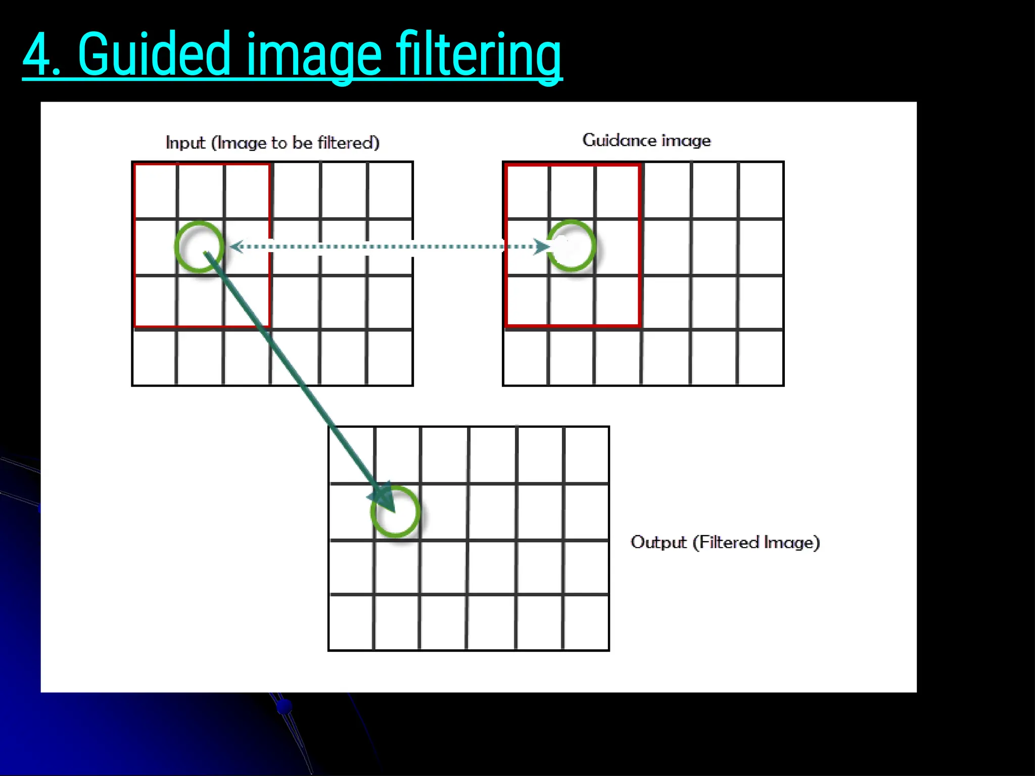
4. Guided imagefiltering ● Guided image filtering uses context from another image, known as a guidance image, to influence the output of image filtering. ● Like other filtering operations, guided image filtering is a neighborhood operation. ● However, guided image filtering takes into account the statistics of a region in the corresponding spatial neighborhood in the guidance image when calculating the value of the output pixel. ● The guidance image can be the image itself, a different version of the image, or a completely different image.
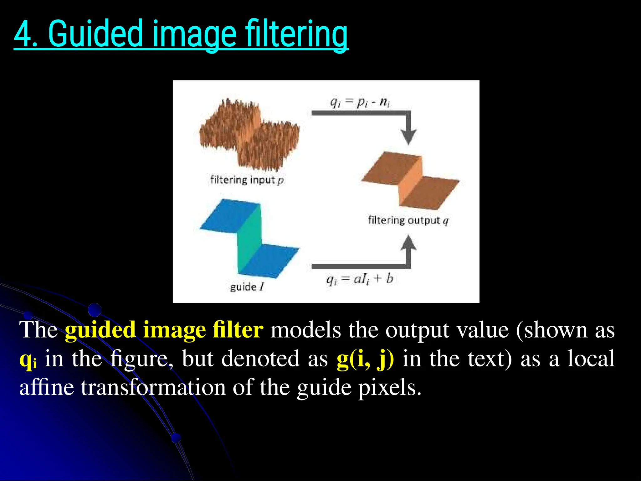
4. Guided imagefiltering The guided image filter models the output value (shown as qi in the figure, but denoted as g(i, j) in the text) as a local affine transformation of the guide pixels.
15.
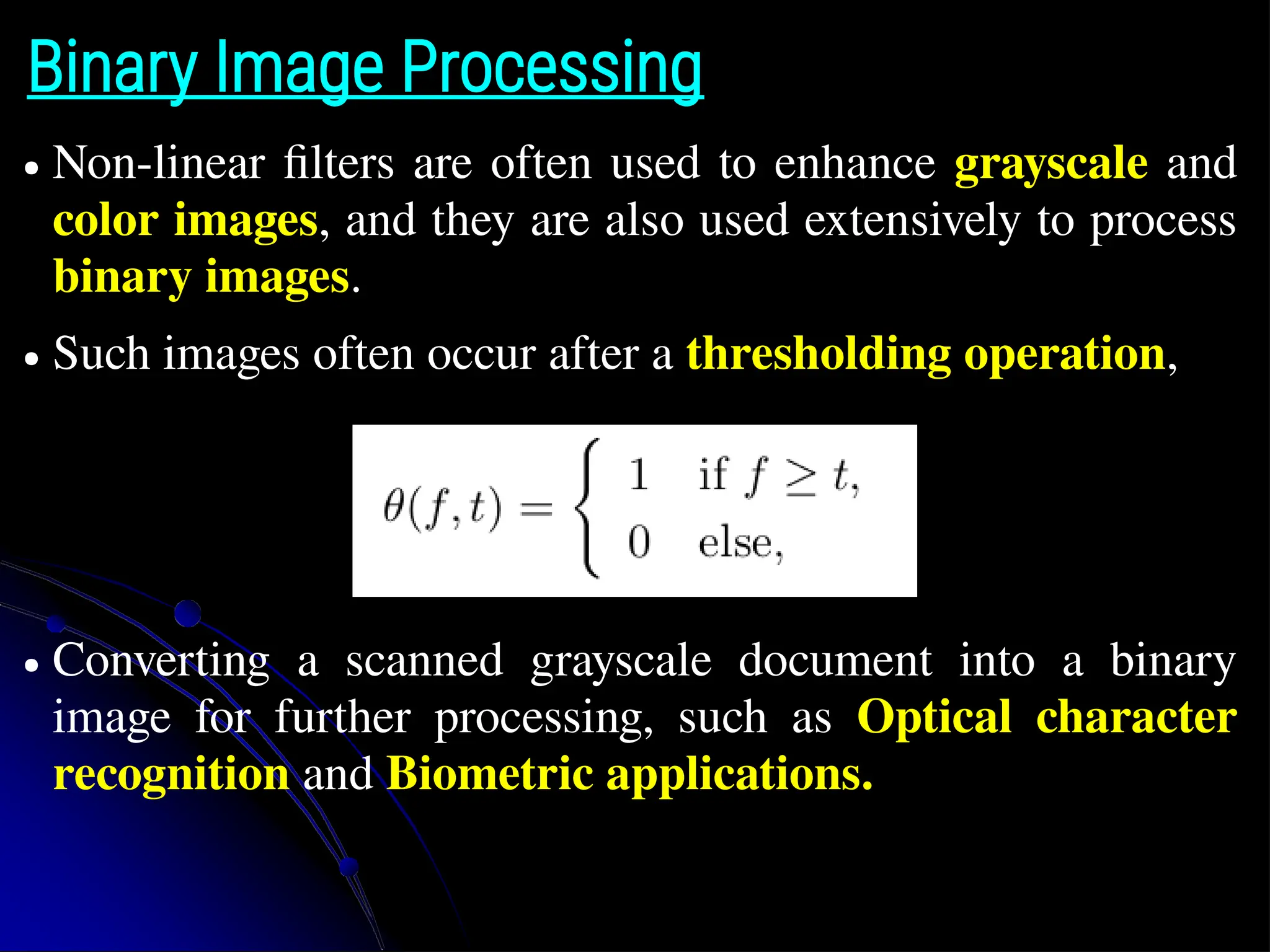
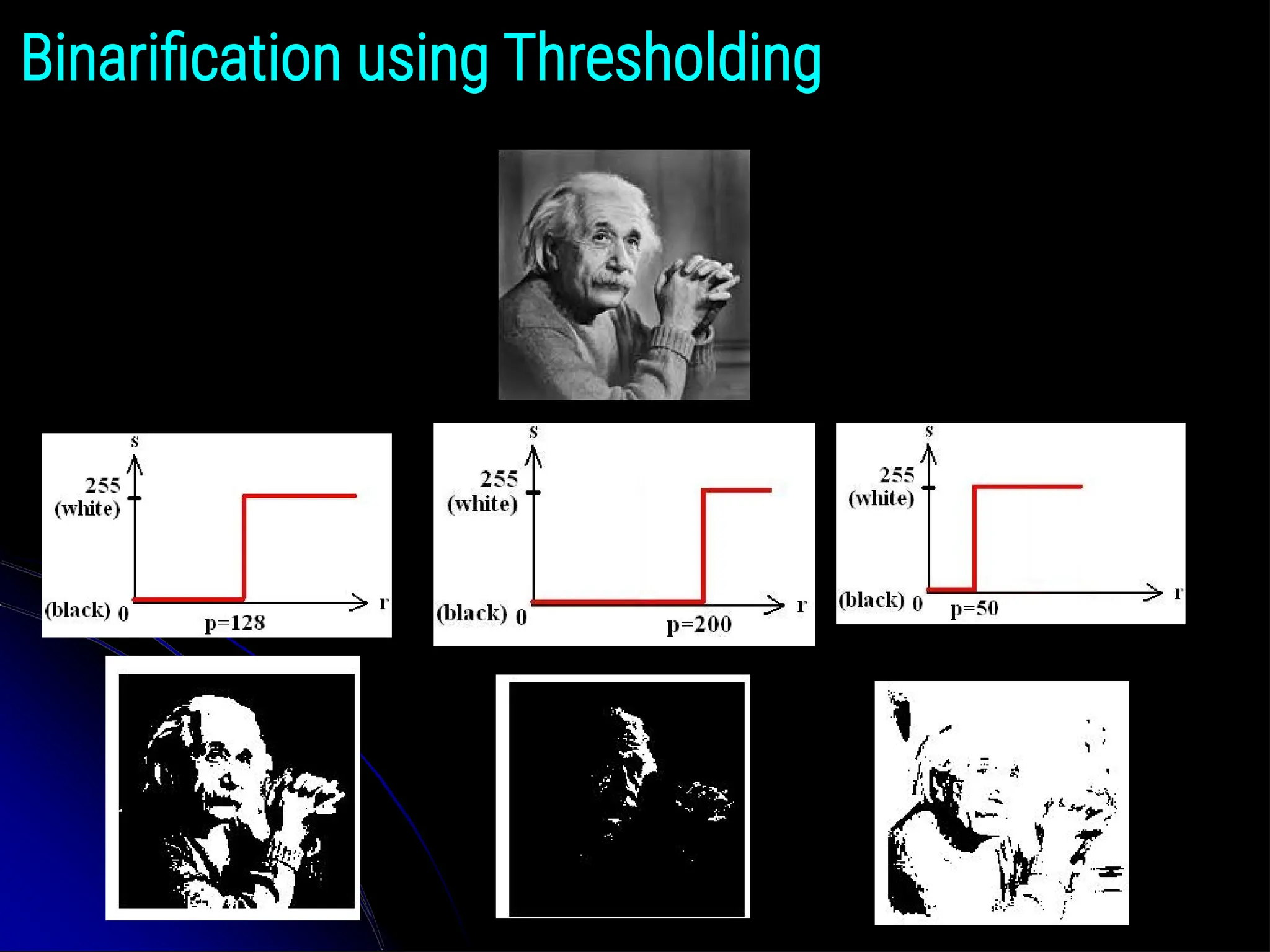
Binary Image Processing ●Non-linear filters are often used to enhance grayscale and color images, and they are also used extensively to process binary images. ● Such images often occur after a thresholding operation, ● Converting a scanned grayscale document into a binary image for further processing, such as Optical character recognition and Biometric applications.
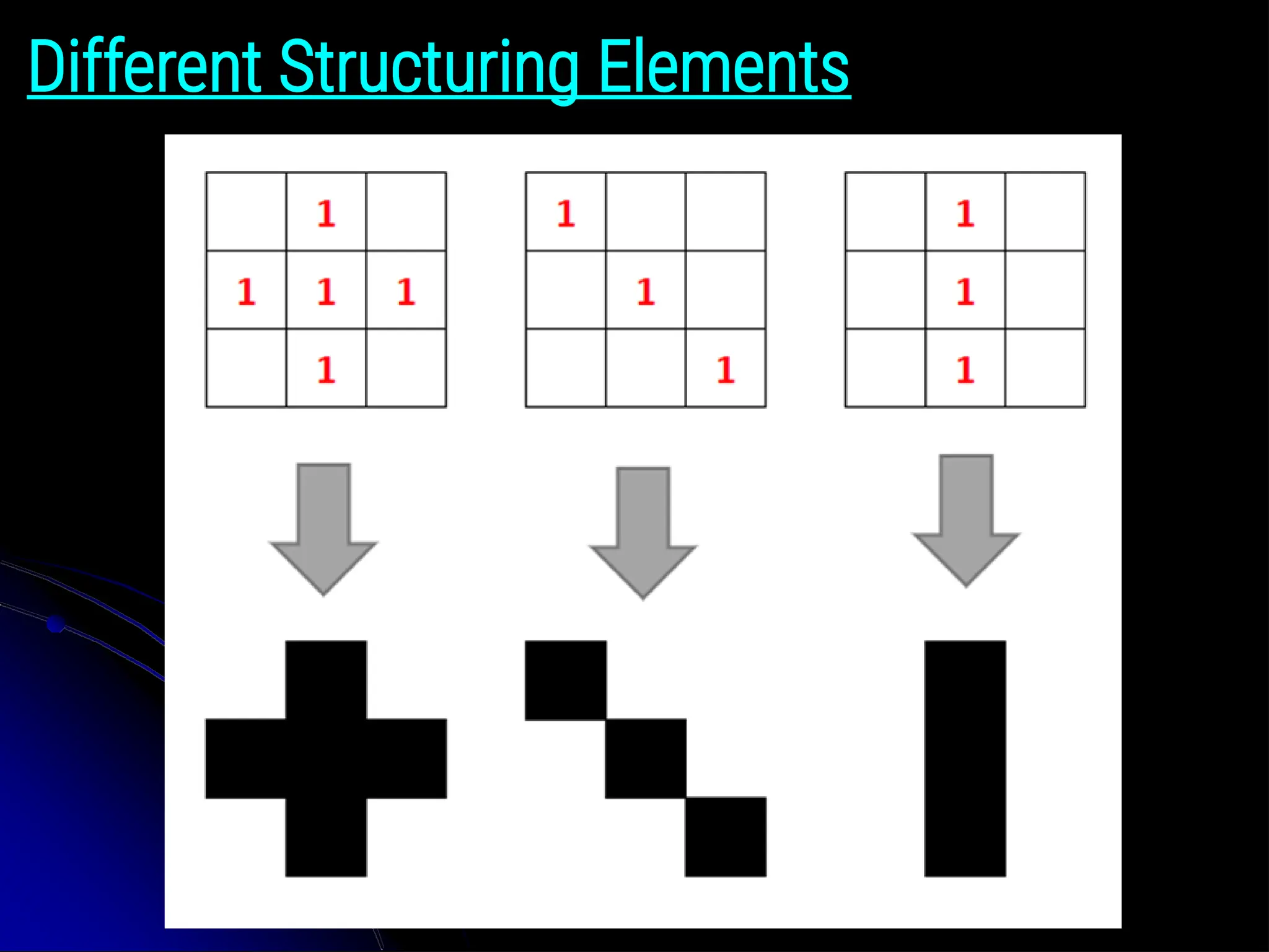
Morphological Operations ● Morphologicaloperations are image processing techniques that change the shape and structure of objects in an image. ● They are based on mathematical morphology, which studies the properties of shapes and patterns. ● To perform such an operation, we first apply convolution on the binary image with a binary structuring element. ● Then select a binary output value depending on the thresholded result of the convolution. ● The structuring element can be any shape, from a simple 3 × 3 box filter, to more complicated disc structures.
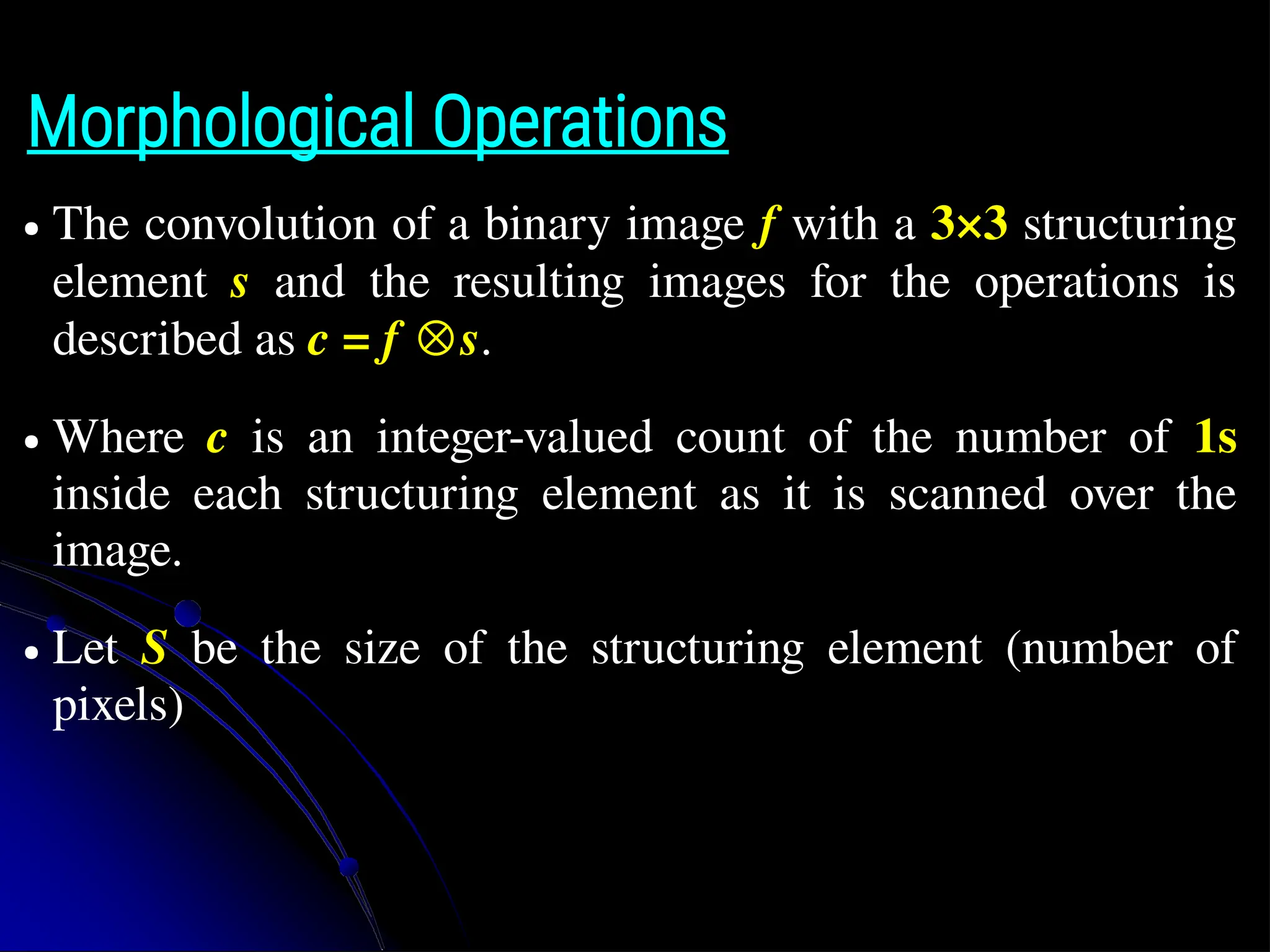
Morphological Operations ● Theconvolution of a binary image f with a 3×3 structuring element s and the resulting images for the operations is described as c = f ⊗s. ● Where c is an integer-valued count of the number of 1s inside each structuring element as it is scanned over the image. ● Let S be the size of the structuring element (number of pixels)
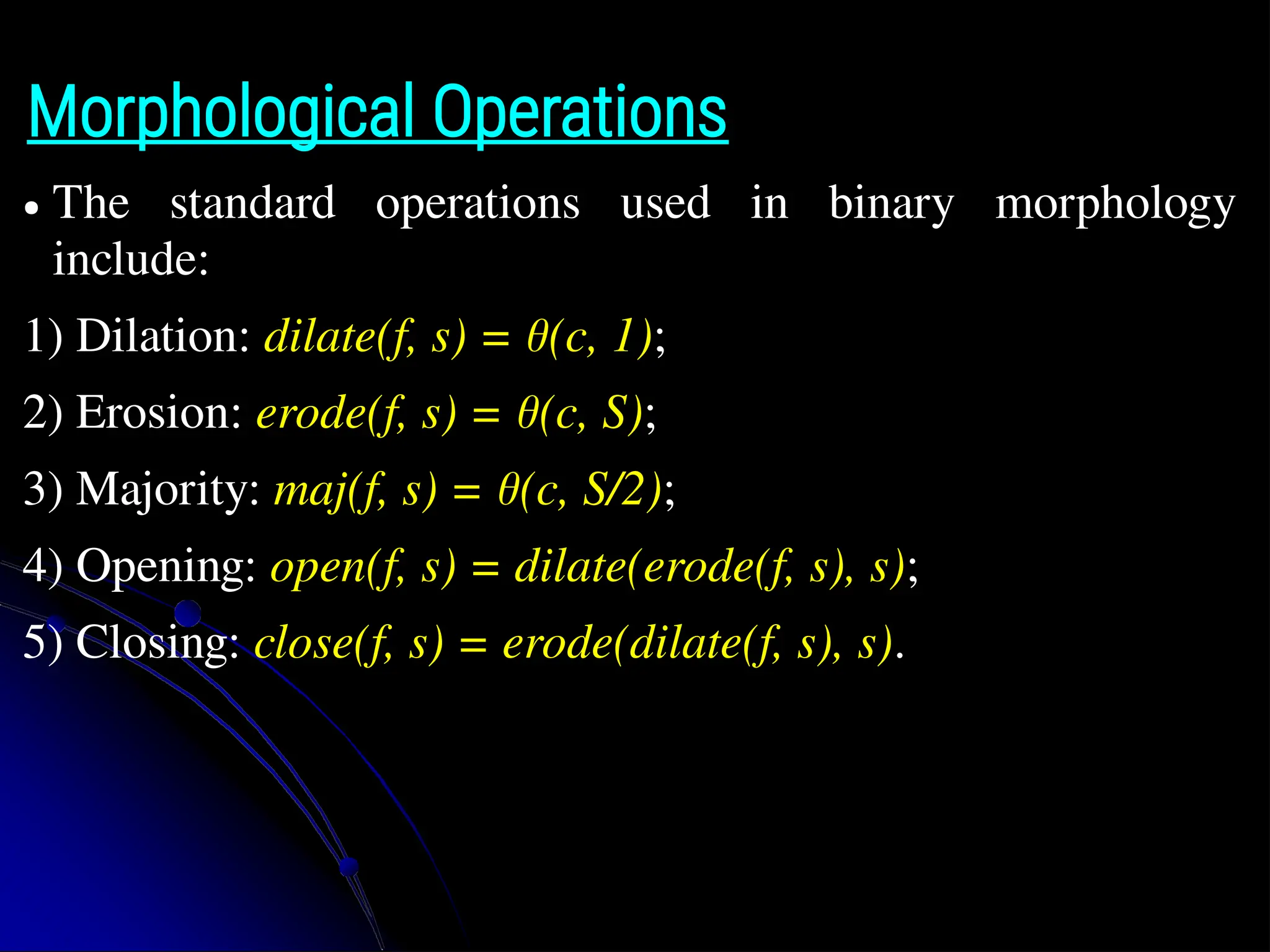
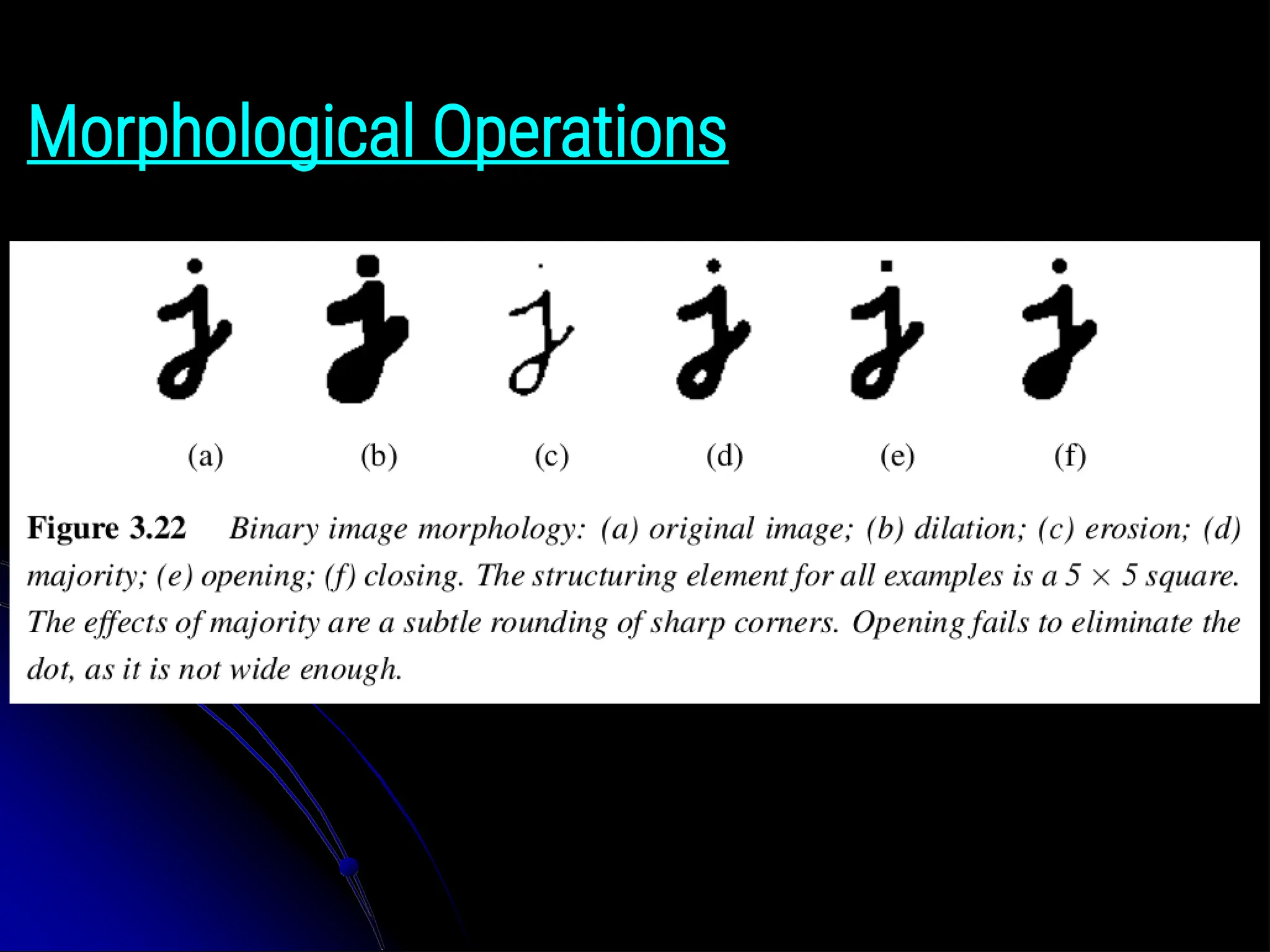
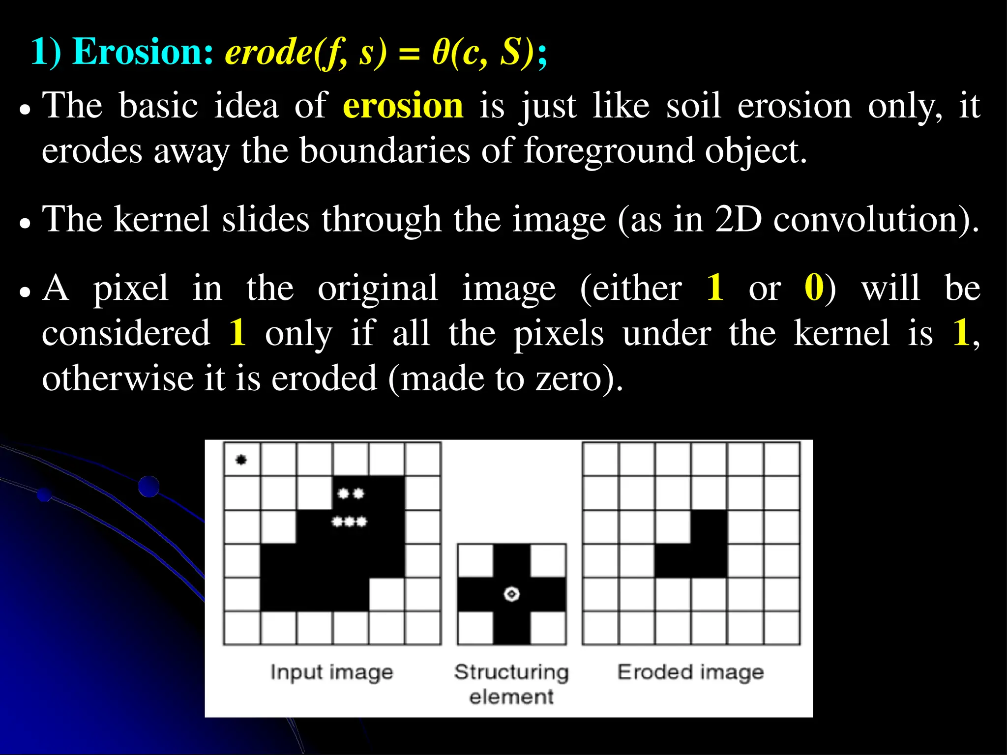
1) Erosion: erode(f,s) = θ(c, S); ● The basic idea of erosion is just like soil erosion only, it erodes away the boundaries of foreground object. ● The kernel slides through the image (as in 2D convolution). ● A pixel in the original image (either 1 or 0) will be considered 1 only if all the pixels under the kernel is 1, otherwise it is eroded (made to zero).
23.
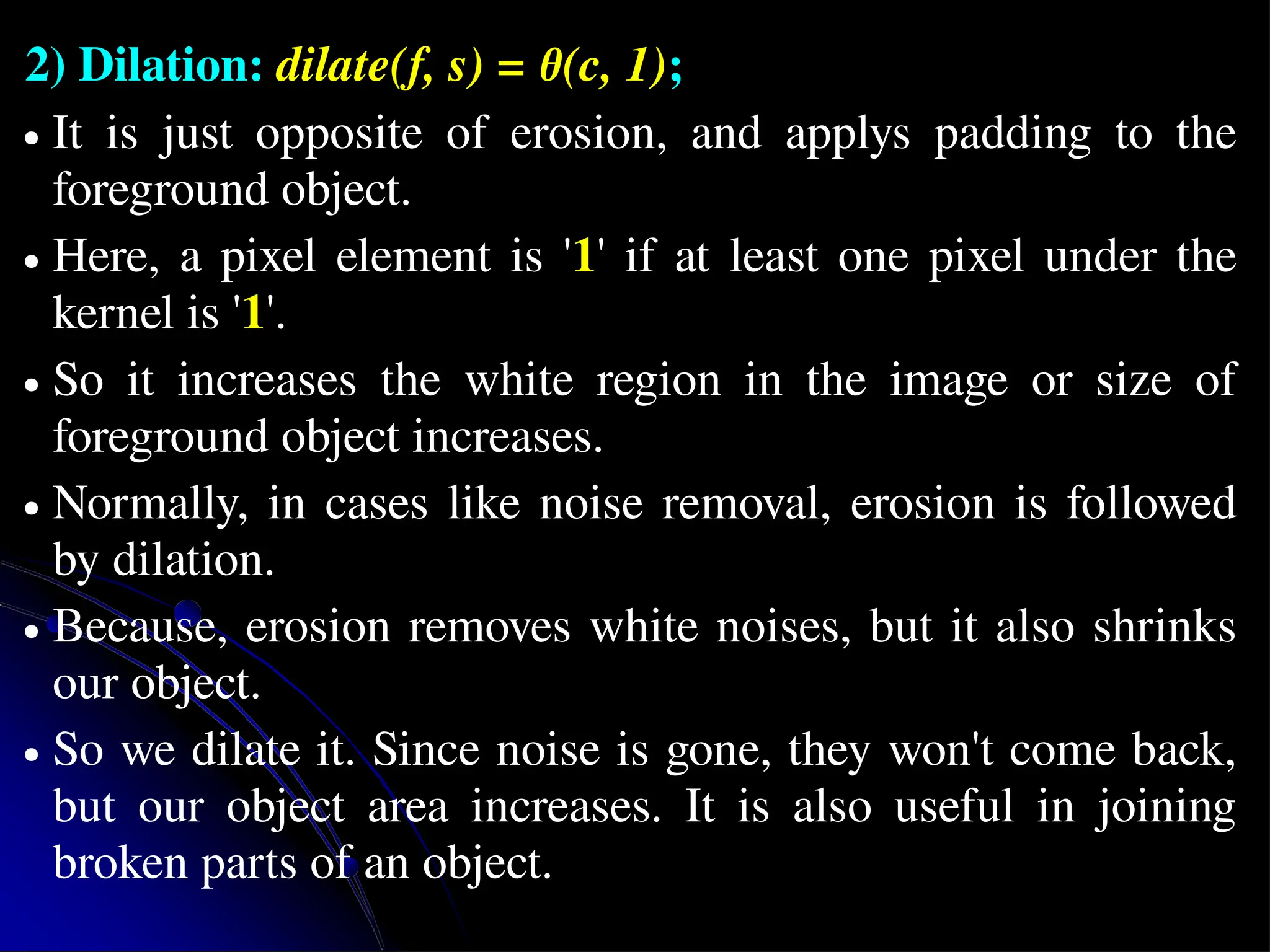
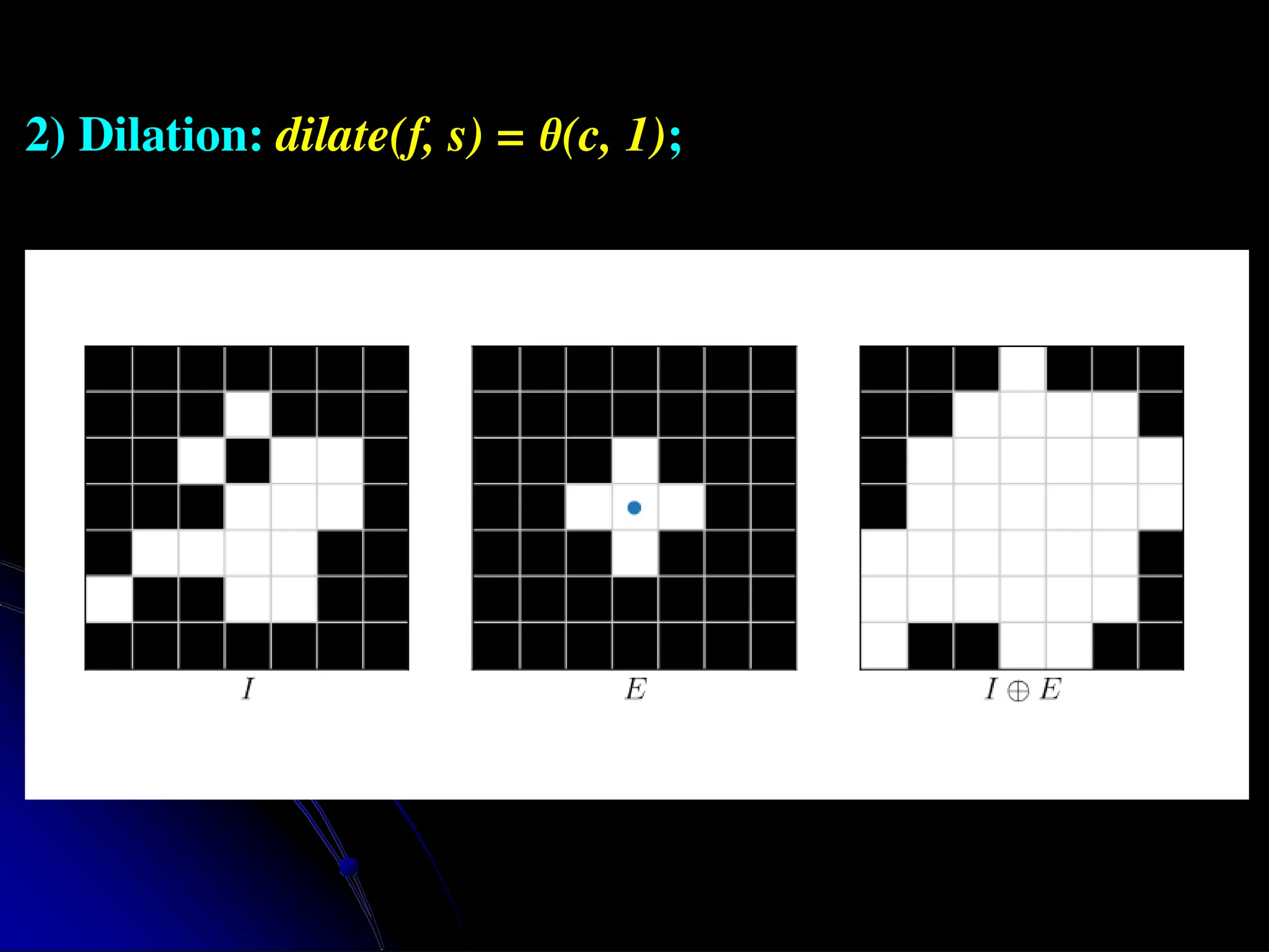
2) Dilation: dilate(f,s) = θ(c, 1); ● It is just opposite of erosion, and applys padding to the foreground object. ● Here, a pixel element is '1' if at least one pixel under the kernel is '1'. ● So it increases the white region in the image or size of foreground object increases. ● Normally, in cases like noise removal, erosion is followed by dilation. ● Because, erosion removes white noises, but it also shrinks our object. ● So we dilate it. Since noise is gone, they won't come back, but our object area increases. It is also useful in joining broken parts of an object.
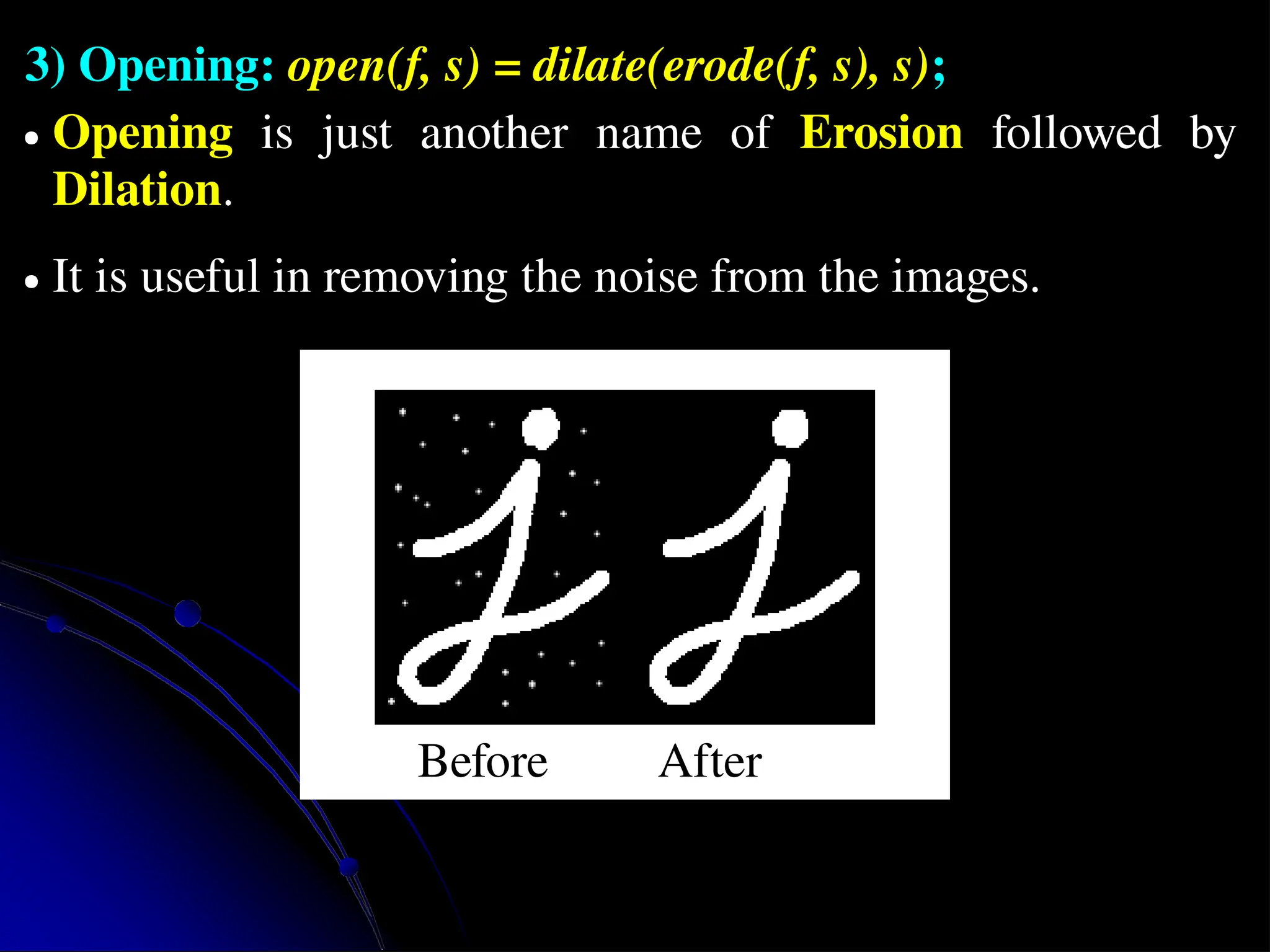
3) Opening: open(f,s) = dilate(erode(f, s), s); ● Opening is just another name of Erosion followed by Dilation. ● It is useful in removing the noise from the images. Before After
26.
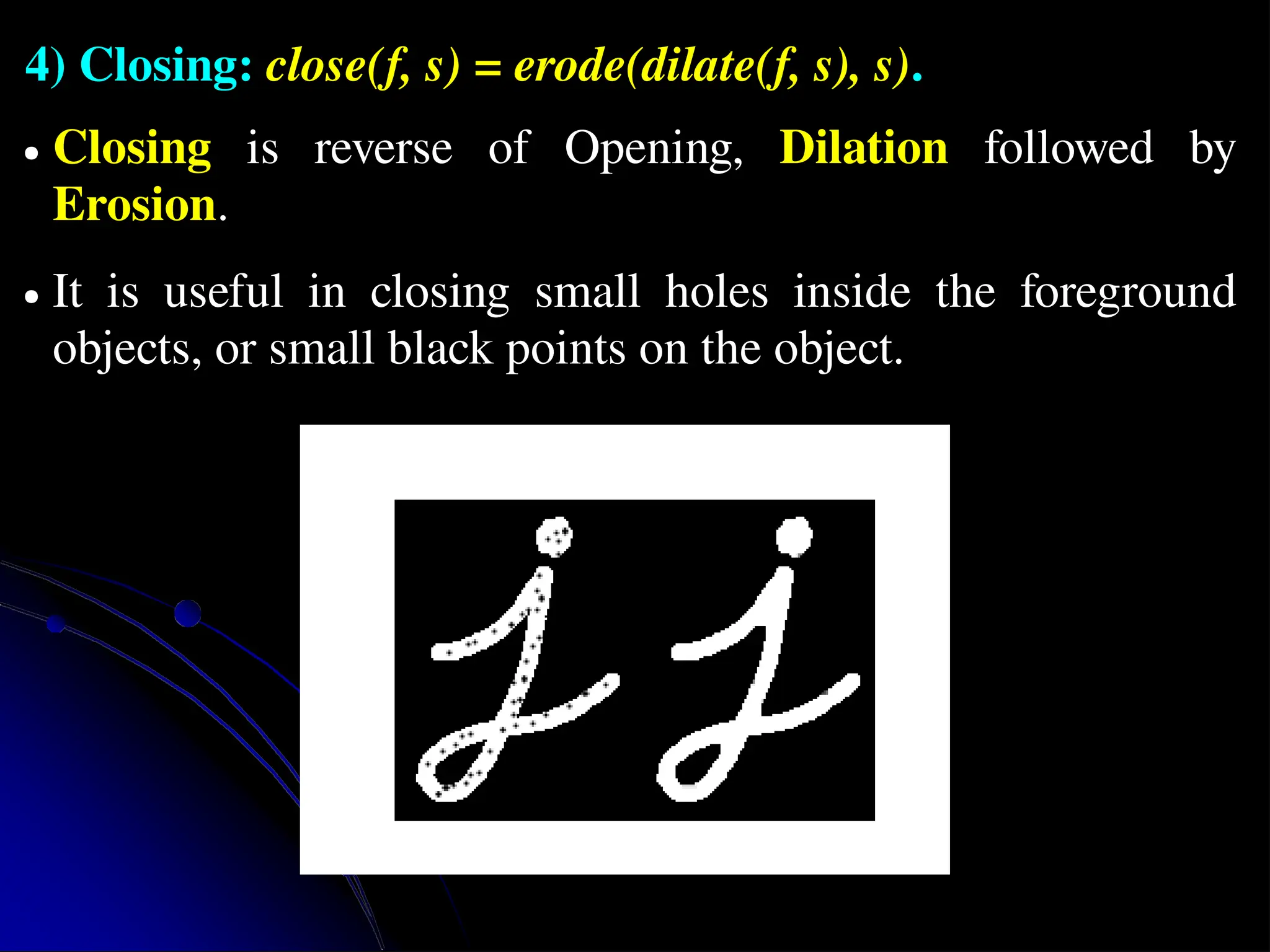
4) Closing: close(f,s) = erode(dilate(f, s), s). ● Closing is reverse of Opening, Dilation followed by Erosion. ● It is useful in closing small holes inside the foreground objects, or small black points on the object.
27.
Distance transforms ● Thedistance transform provides a metric or measure of the separation of points in the image. ● The distance transform is useful in quickly computing the distance between a point and a set of points or a curve using a two-pass raster algorithm. ● It has many applications, including level sets, binary image alignment, feathering in image stitching and blending, and nearest point alignment.
28.
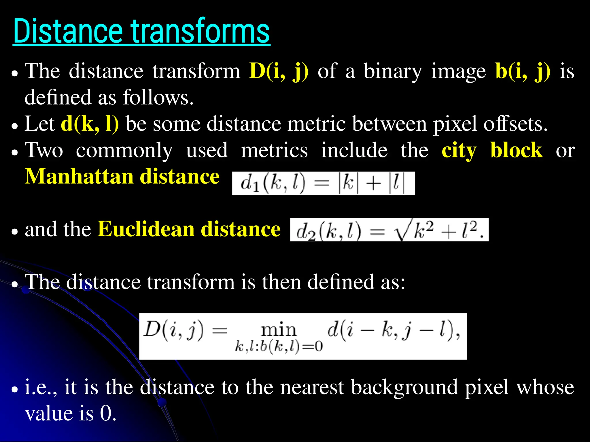
Distance transforms ● Thedistance transform D(i, j) of a binary image b(i, j) is defined as follows. ● Let d(k, l) be some distance metric between pixel offsets. ● Two commonly used metrics include the city block or Manhattan distance ● and the Euclidean distance ● The distance transform is then defined as: ● i.e., it is the distance to the nearest background pixel whose value is 0.
29.
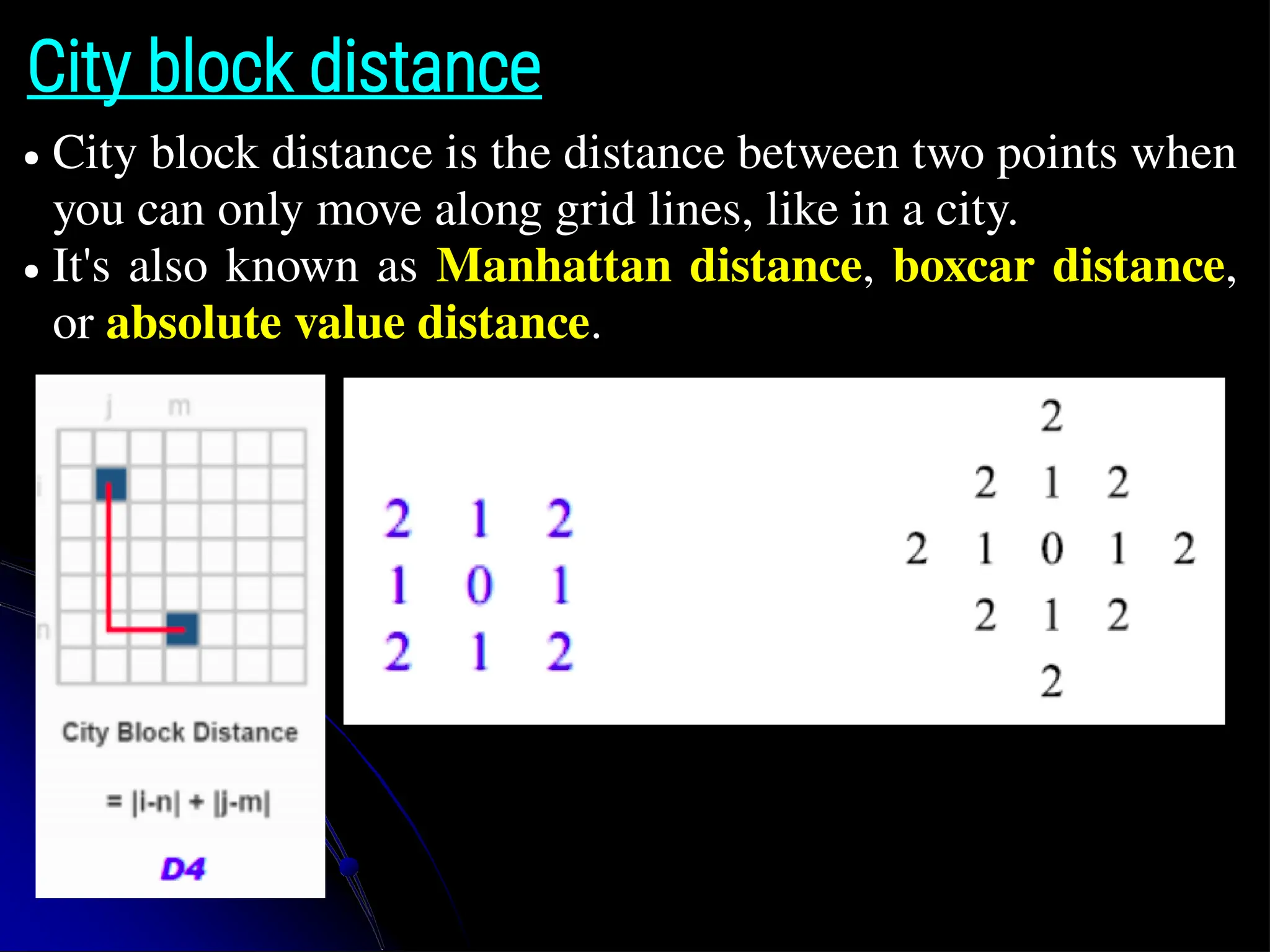
City block distance ●City block distance is the distance between two points when you can only move along grid lines, like in a city. ● It's also known as Manhattan distance, boxcar distance, or absolute value distance.
30.
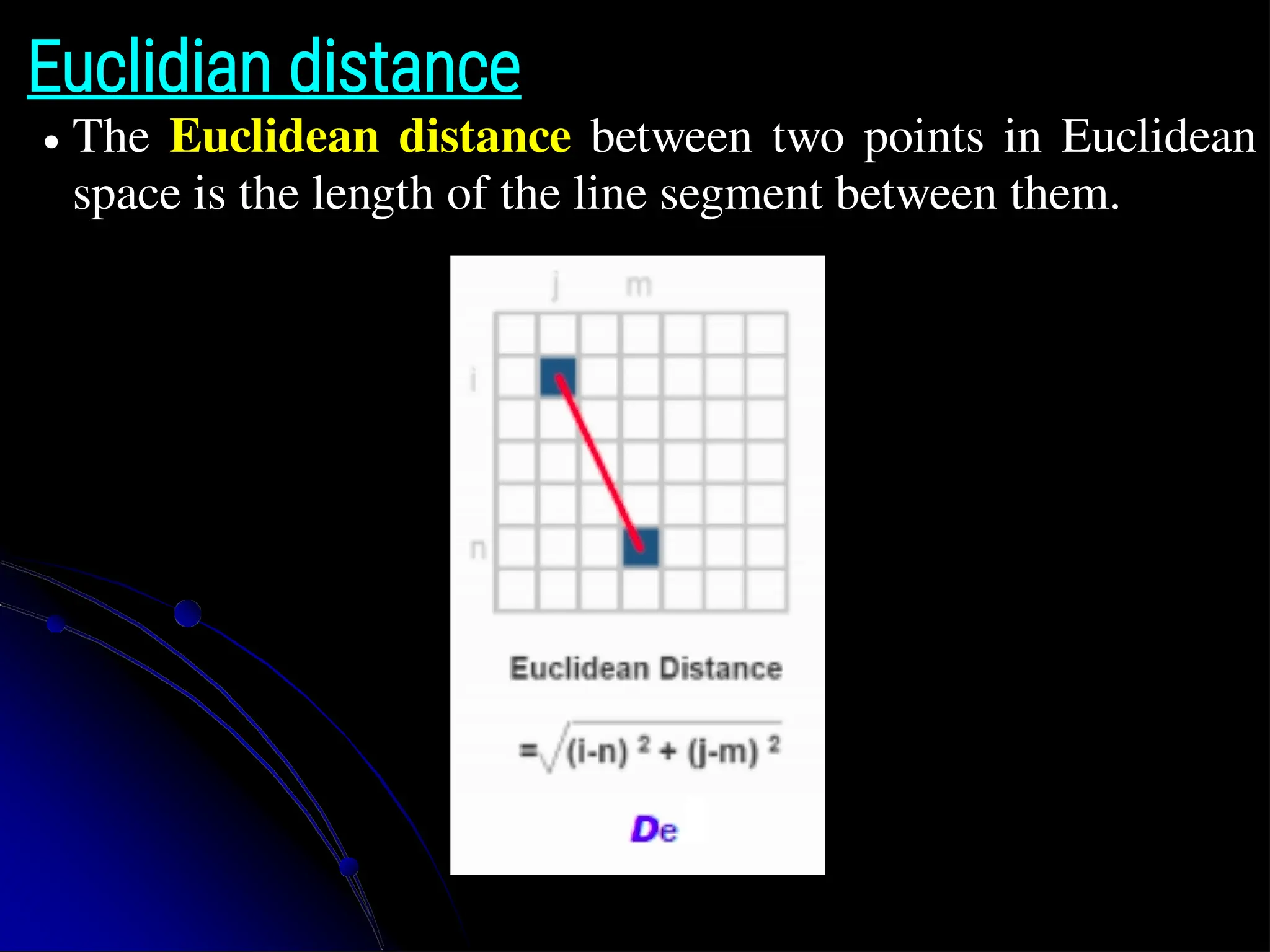
Euclidian distance ● TheEuclidean distance between two points in Euclidean space is the length of the line segment between them.
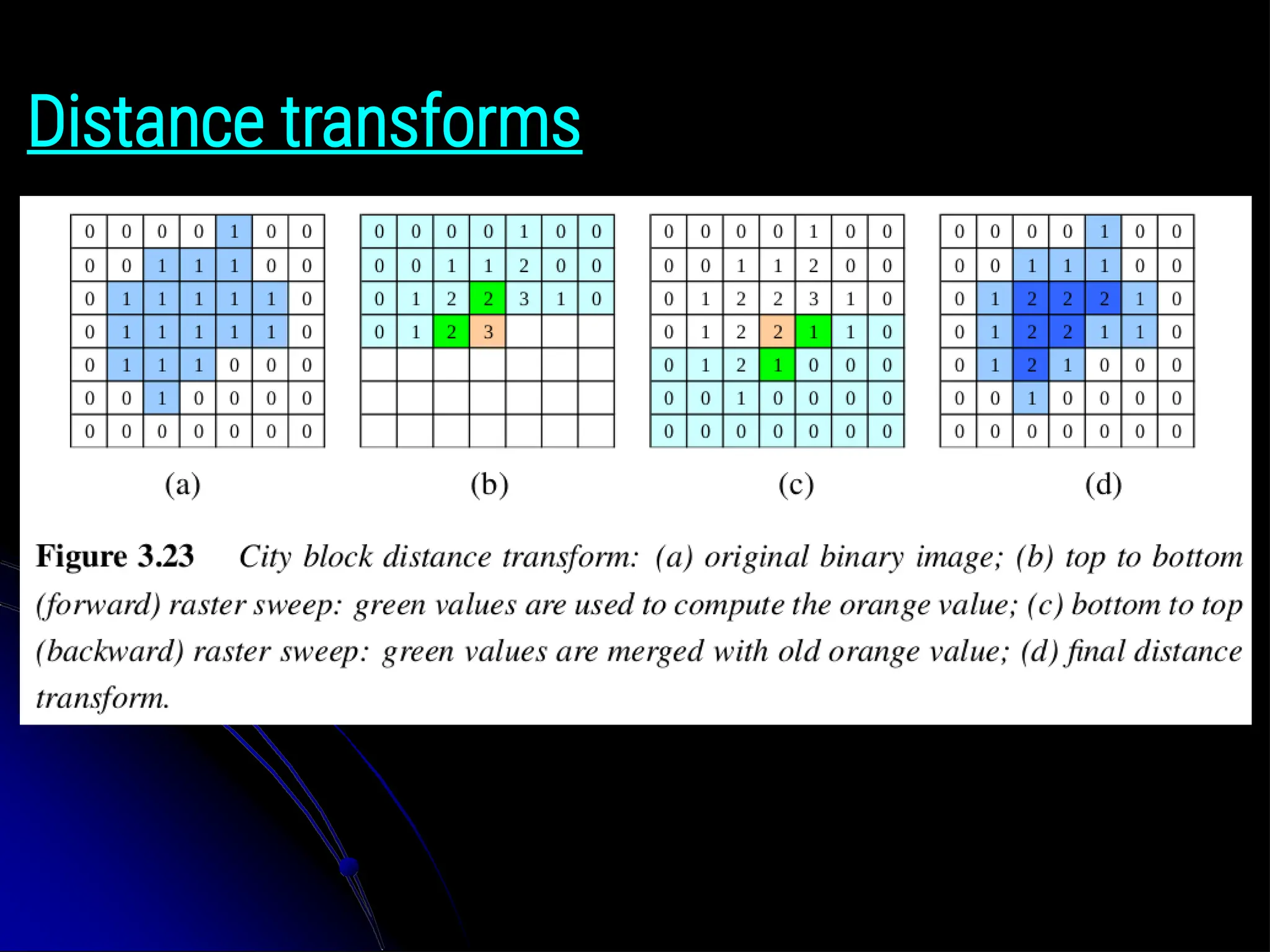
Distance transforms ● TheD1 city block distance transform can be efficiently computed using a forward and backward pass of a simple raster-scan algorithm. ● During the forward pass, each non-zero pixel in b is replaced by the minimum of 1 + the distance of its north orwest neighbor. ● During the backward pass, the same occurs, except that the minimum is both over the current value D and 1 + the distance of the south and east neighbors.
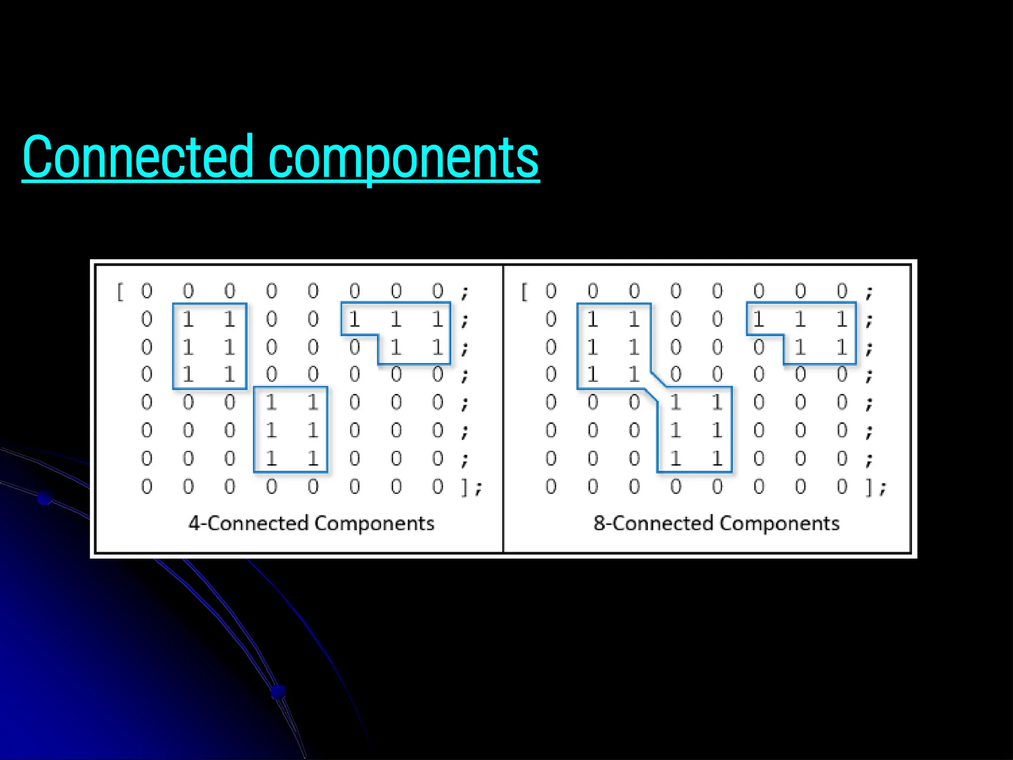
Connected components ● Anotheruseful semi-global image operation is finding connected components, which are defined as regions of adjacent pixels that have the same input value or label. ● Pixels are said to be N4 adjacent if they are immediately horizontally or vertically adjacent, and N8 if they can also be diagonally adjacent. ● Both variants of connected components are widely used in a variety of applications, such as finding individual letters in a scanned document or finding objects (say, cells) in a thresholded image and computing their area statistics.
35.
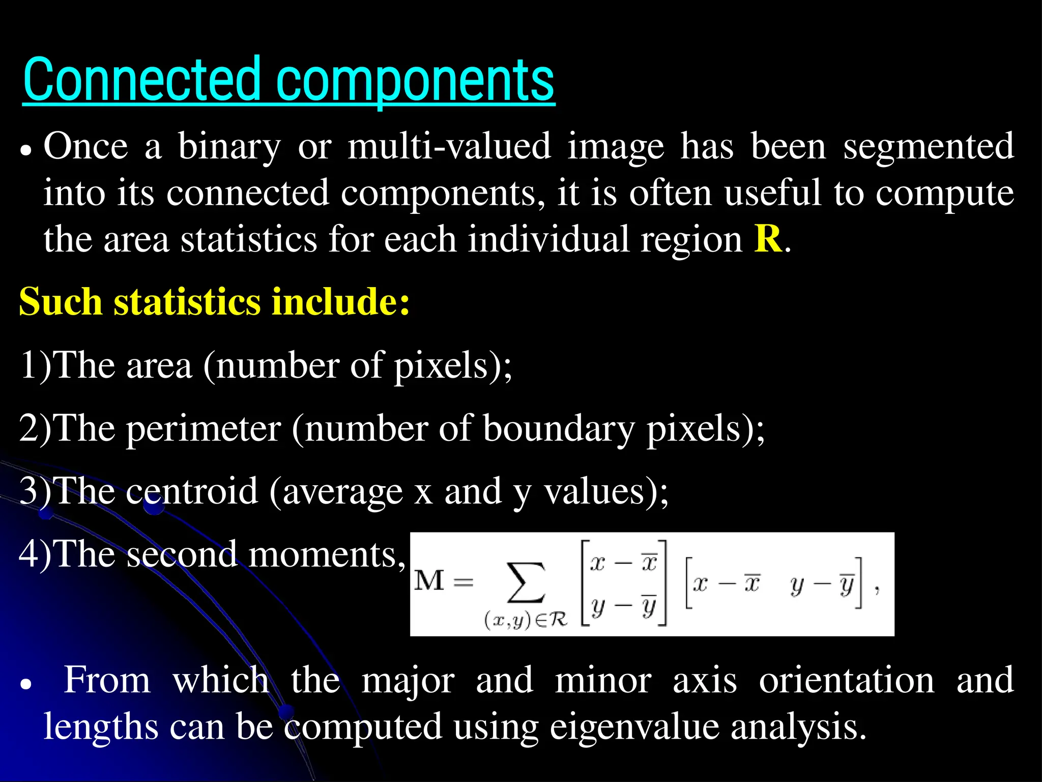
Connected components ● Oncea binary or multi-valued image has been segmented into its connected components, it is often useful to compute the area statistics for each individual region R. Such statistics include: 1)The area (number of pixels); 2)The perimeter (number of boundary pixels); 3)The centroid (average x and y values); 4)The second moments, ● From which the major and minor axis orientation and lengths can be computed using eigenvalue analysis.
36.
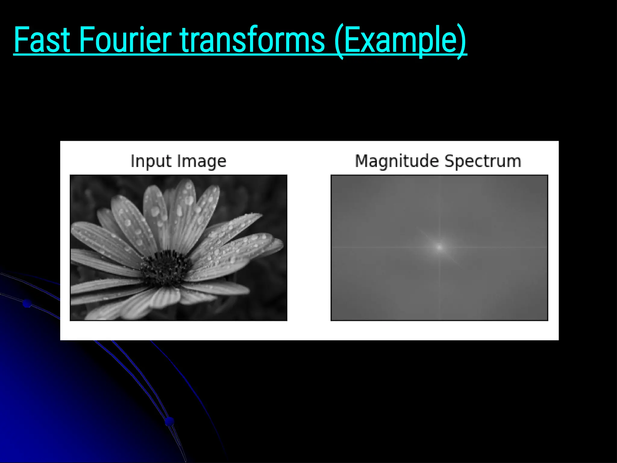
Fourier transforms ● Fourieranalysis could be used to analyze the frequency characteristics of various signals. ● In this section, we explain both how Fourier analysis lets us to determine these characteristics (i.e., the frequency content of an image). ● And also how the Fast Fourier Transform (FFT) lets us to perform large-kernel convolutions in time-independent of the kernel’s size.
37.
Image Operations inDifferent Domains 1) Gray value (histogram) domain ● Histogram stretching, equalization, specification, etc... 2) Spatial (image) domain ● Average filter, median filter, gradient, Laplacian, etc… 3) Frequency (Fourier) domain ● Fast Fourier Transform, Wavelets etc...
38.
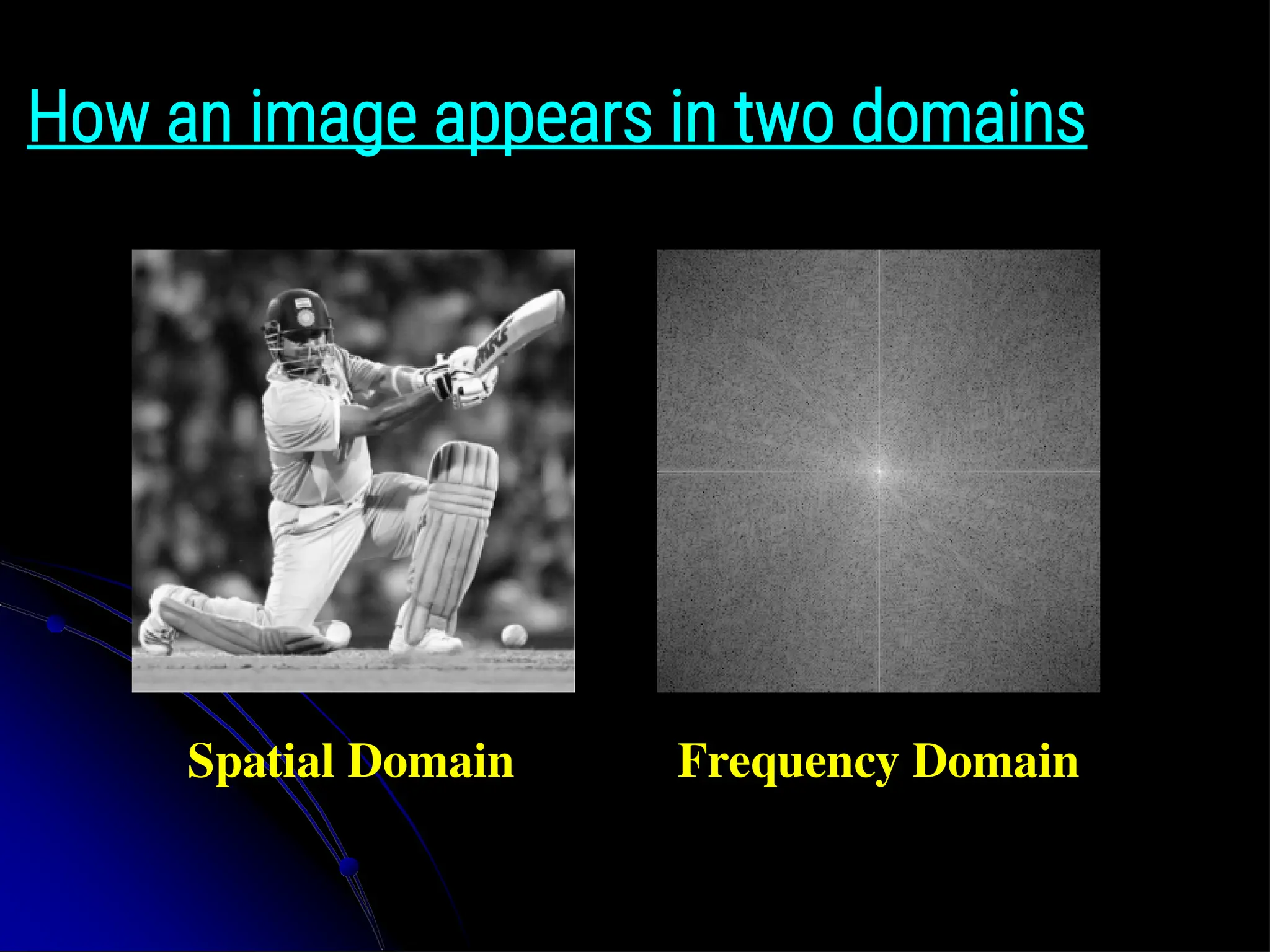
Fourier transforms ● TheFourier Transform is an important image processing tool which is used to decompose an image into its sine and cosine components. ● The output of the transformation represents the image in the Fourier or frequency domain, while the input image is the spatial domain equivalent. ● In the Fourier domain image, each point represents a particular frequency contained in the spatial domain image. ● The Fourier Transform is used in a wide range of applications, such as image analysis, image filtering, image reconstruction and image compression.
39.
How an imageappears in two domains Spatial Domain Frequency Domain
40.
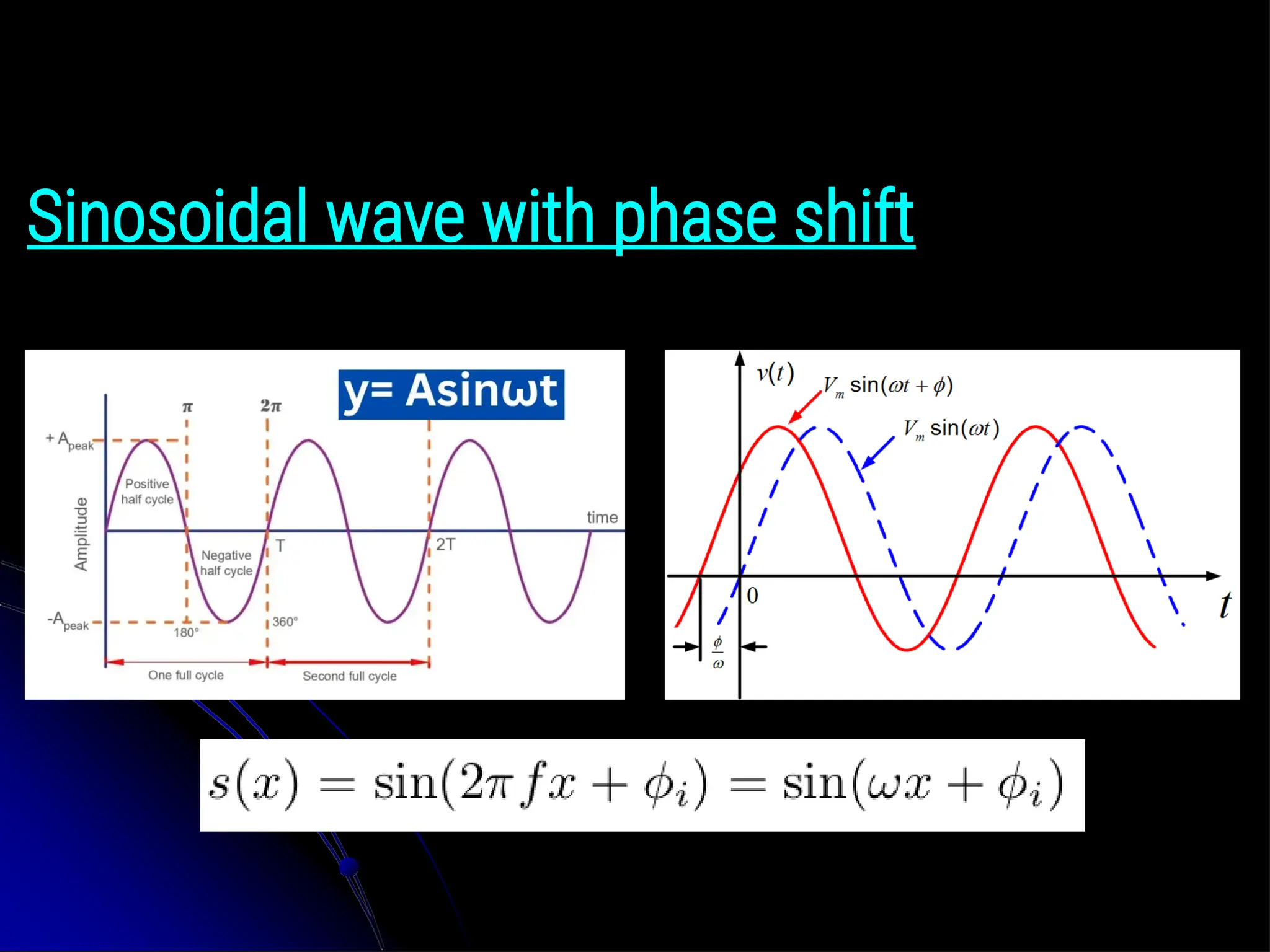
Basics of Fouriertransforms ● For a sinusoidal signal, ● where f is the frequency of signal, and if its frequency domain is taken, we can see a spike at f, and angular frequency ω = 2πf, and phase φi. ● If signal is sampled to form a discrete signal, we get the same frequency domain, but is periodic in the range [-π, π], or [0, 2π] or [0, N] in for N-point DFT). ● You can consider an image as a signal which is sampled in two directions. ● So taking Fourier transform in both X and Y directions gives you the frequency representation of image.
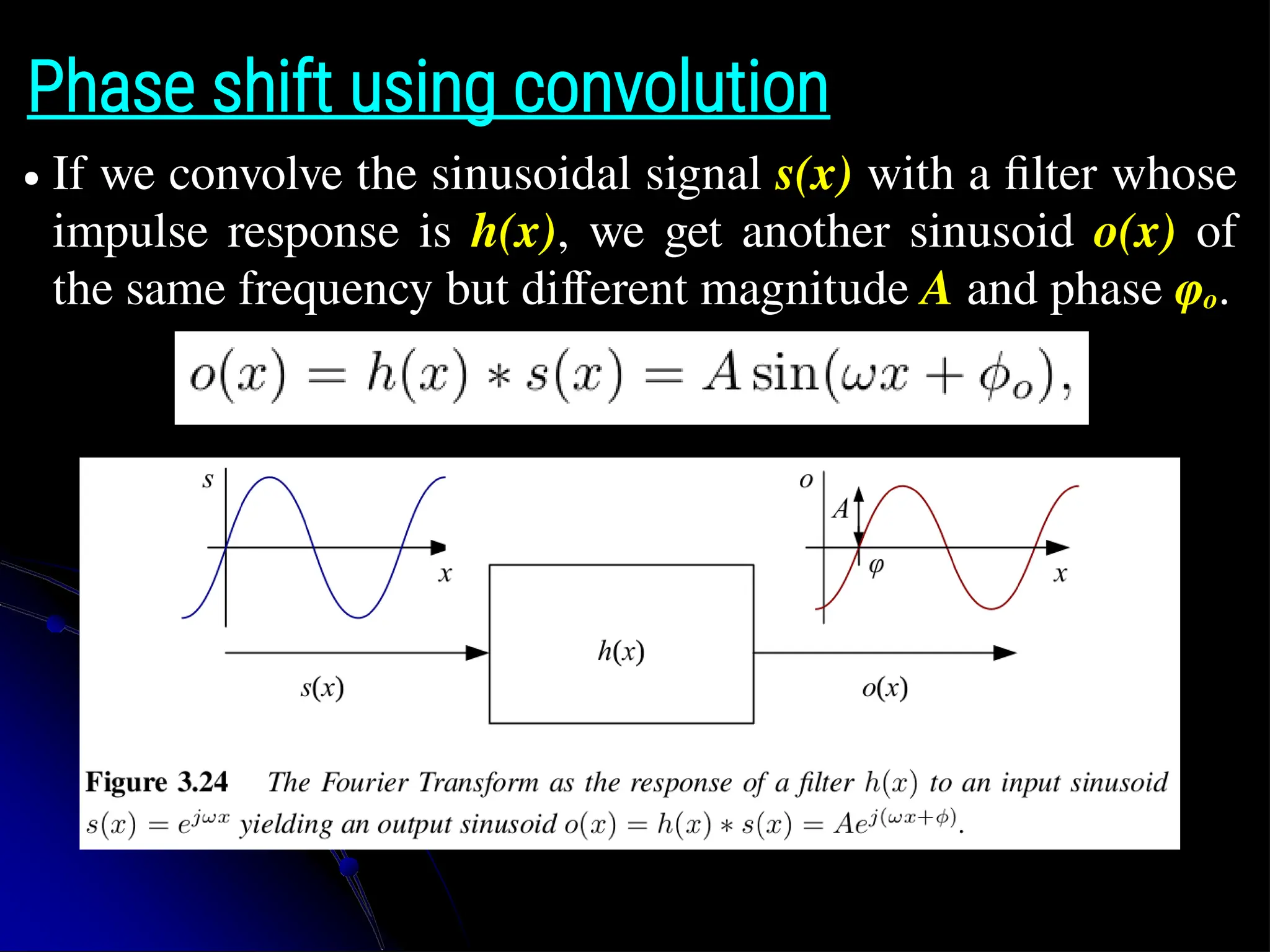
Phase shift usingconvolution ● If we convolve the sinusoidal signal s(x) with a filter whose impulse response is h(x), we get another sinusoid o(x) of the same frequency but different magnitude A and phase φo.
43.
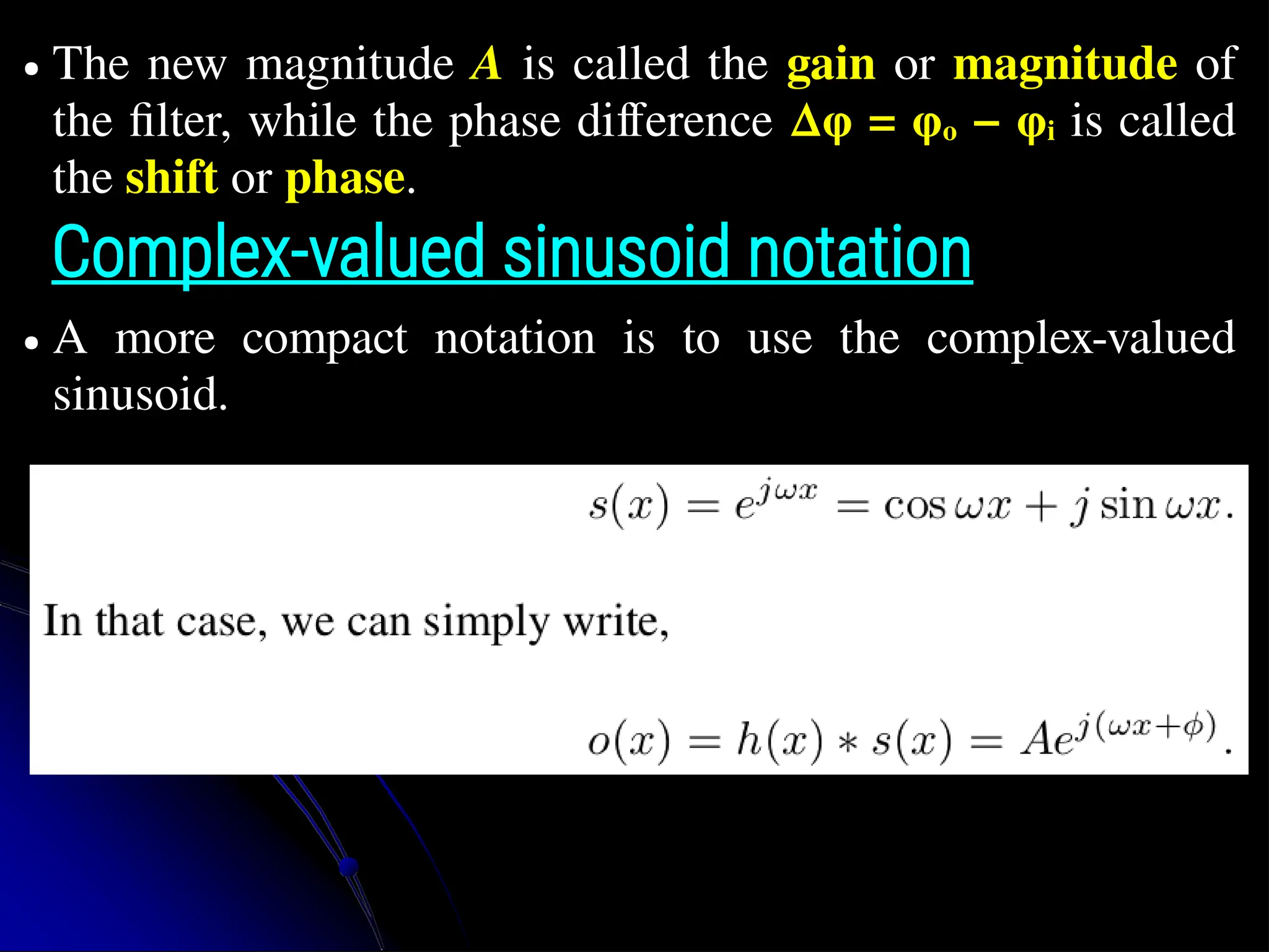
● The newmagnitude A is called the gain or magnitude of the filter, while the phase difference ∆φ = φo − φi is called the shift or phase. Complex-valued sinusoid notation ● A more compact notation is to use the complex-valued sinusoid.
44.
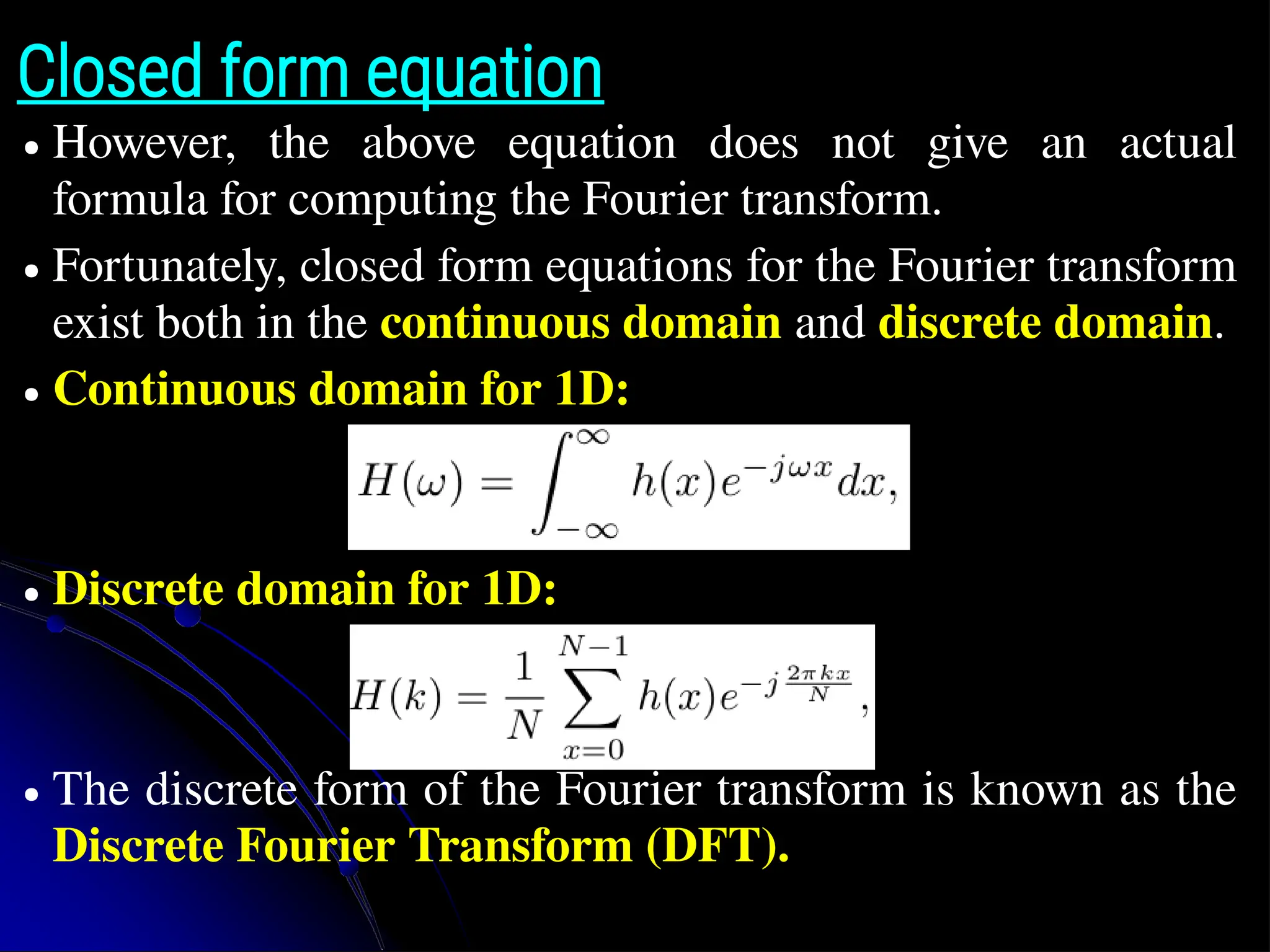
Closed form equation ●However, the above equation does not give an actual formula for computing the Fourier transform. ● Fortunately, closed form equations for the Fourier transform exist both in the continuous domain and discrete domain. ● Continuous domain for 1D: ● Discrete domain for 1D: ● The discrete form of the Fourier transform is known as the Discrete Fourier Transform (DFT).
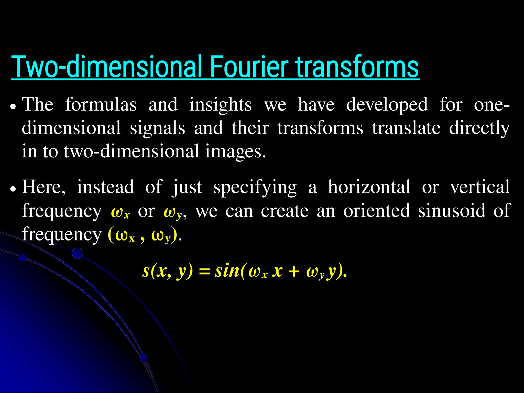
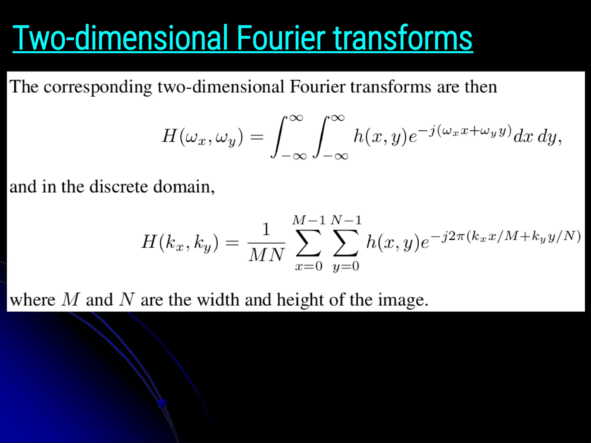
Two-dimensional Fourier transforms ●The formulas and insights we have developed for one- dimensional signals and their transforms translate directly in to two-dimensional images. ● Here, instead of just specifying a horizontal or vertical frequency ωx or ωy, we can create an oriented sinusoid of frequency (ωx , ωy). s(x, y) = sin(ωx x + ωy y).
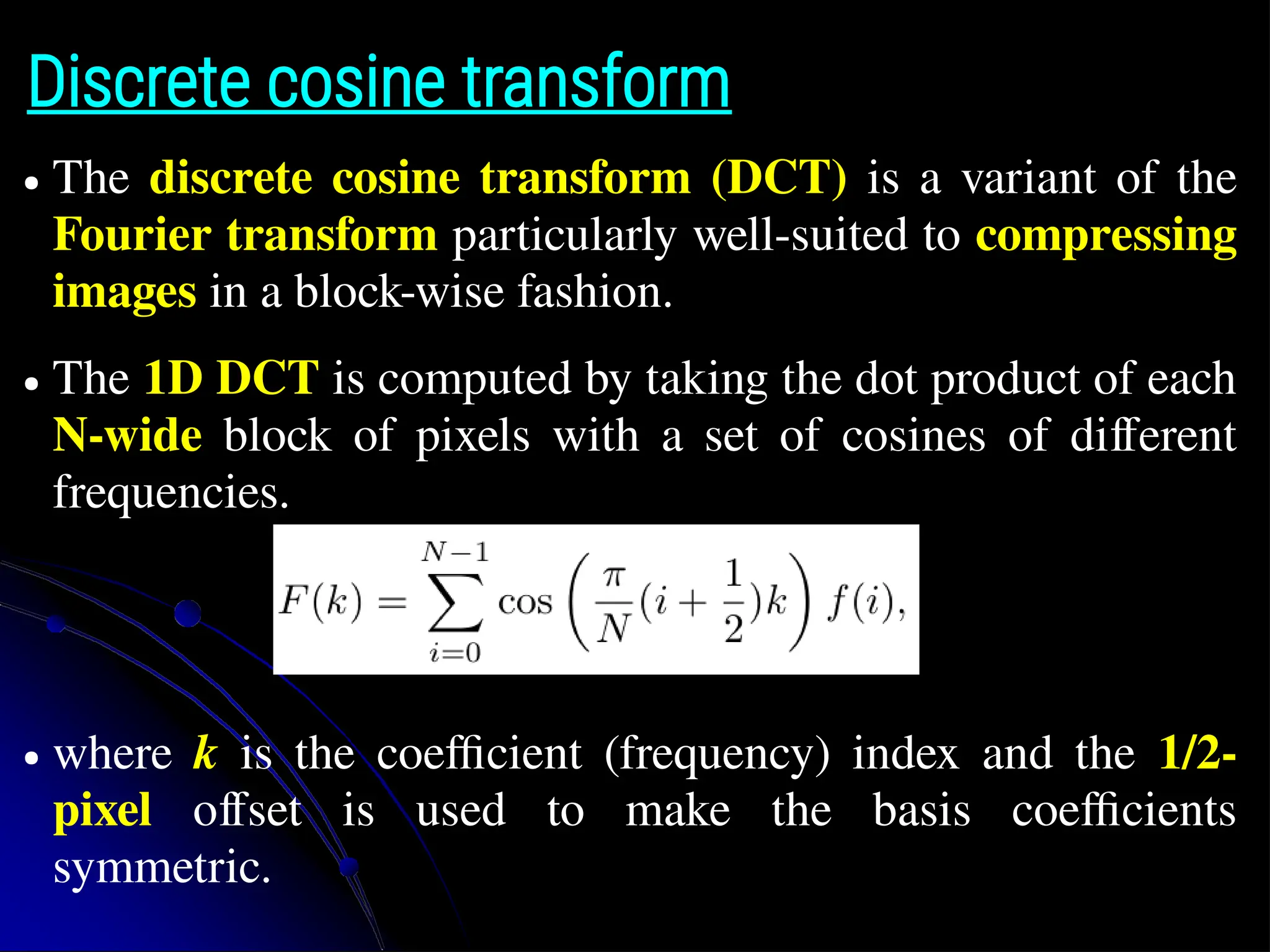
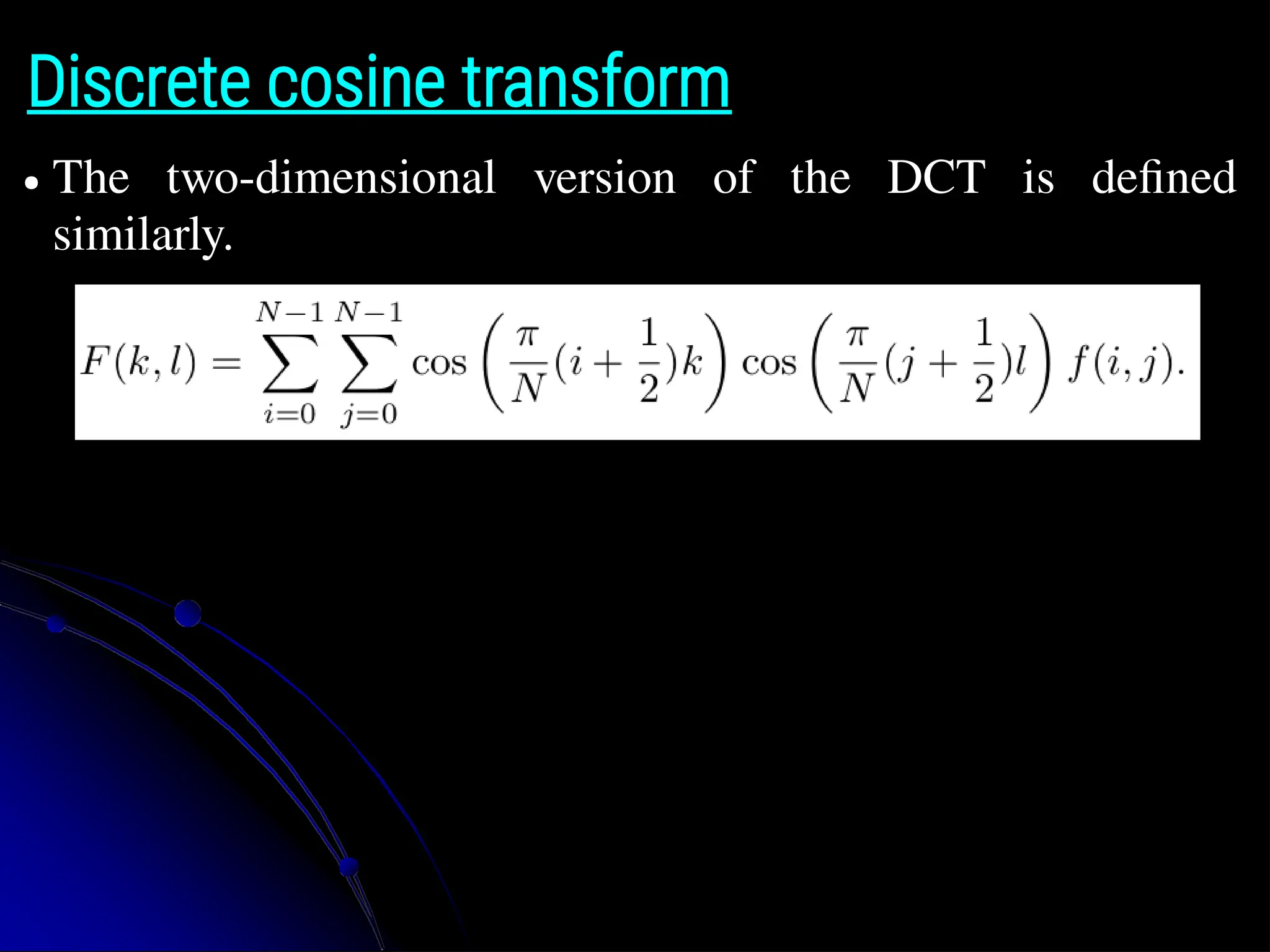
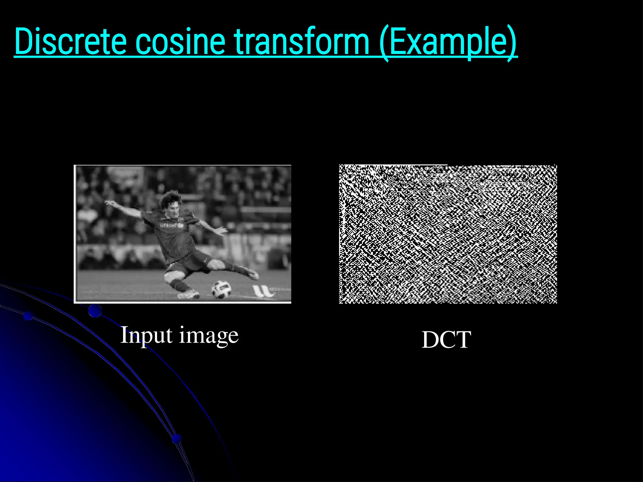
Discrete cosine transform ●The discrete cosine transform (DCT) is a variant of the Fourier transform particularly well-suited to compressing images in a block-wise fashion. ● The 1D DCT is computed by taking the dot product of each N-wide block of pixels with a set of cosines of different frequencies. ● where k is the coefficient (frequency) index and the 1/2- pixel offset is used to make the basis coefficients symmetric.
Applications: Sharpening, blur, andnoise removal ● Another common application of image processing is the enhancement of images through the use of sharpening and noise removal operations, which require some kind of neighborhood processing. ● Traditionally, these kinds of operations were performed using linear filtering.
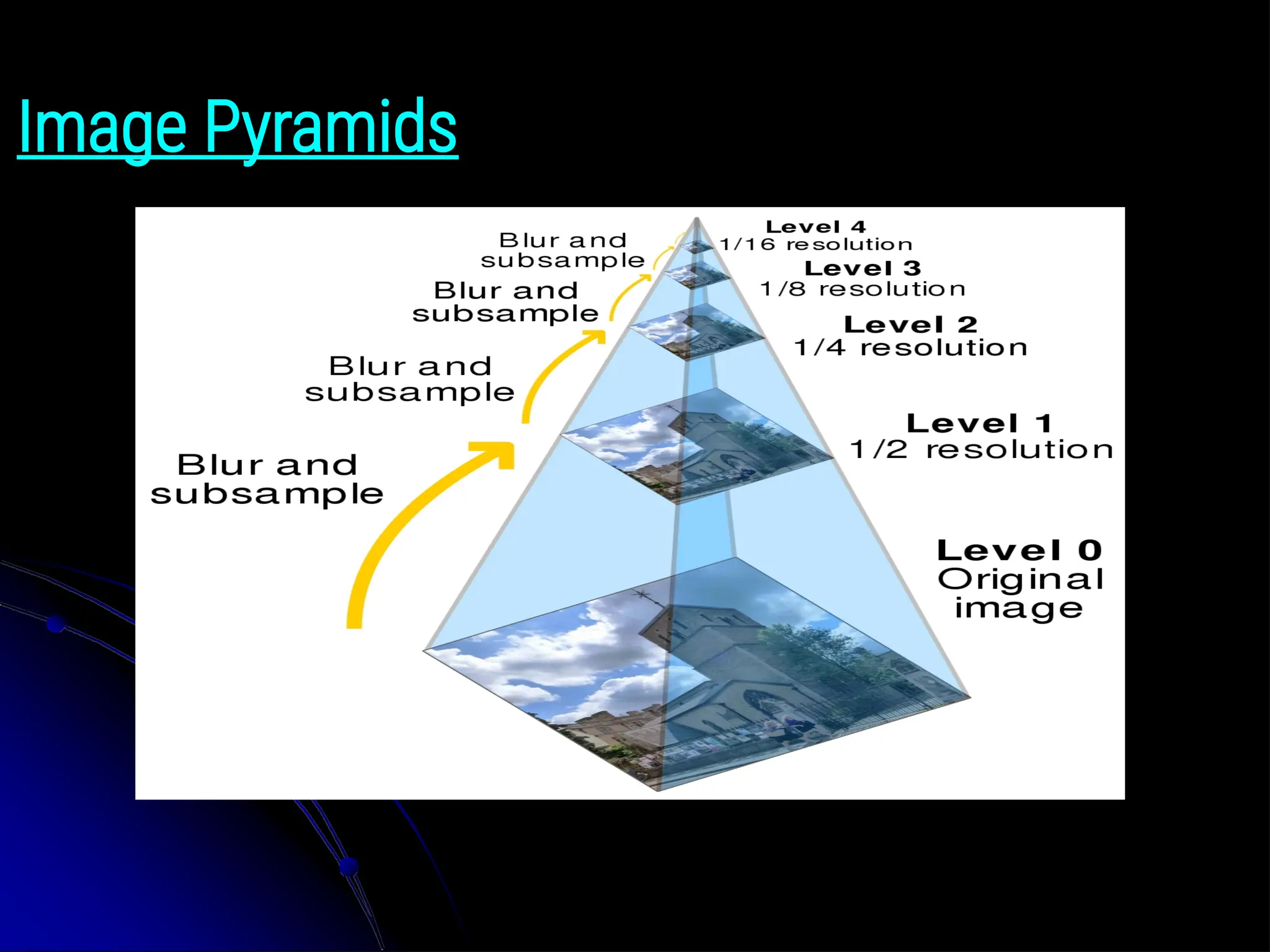
Image Pyramids ● Weoften used to work with an image of constant size. But on some occasions, we need to work with the same image in different resolution. ● For example, we may need to enlarge a small image to increse its resolution for better quality. ● Alternatively, we may want to reduce the size of an image to speed up the execution of an algorithm or to save on storage space or transmission time. ● The set of images with different resolutions are called Image Pyramids (because when they are kept in a stack with the highest resolution image at the bottom and the lowest resolution image at top, it looks like a pyramid).
58.
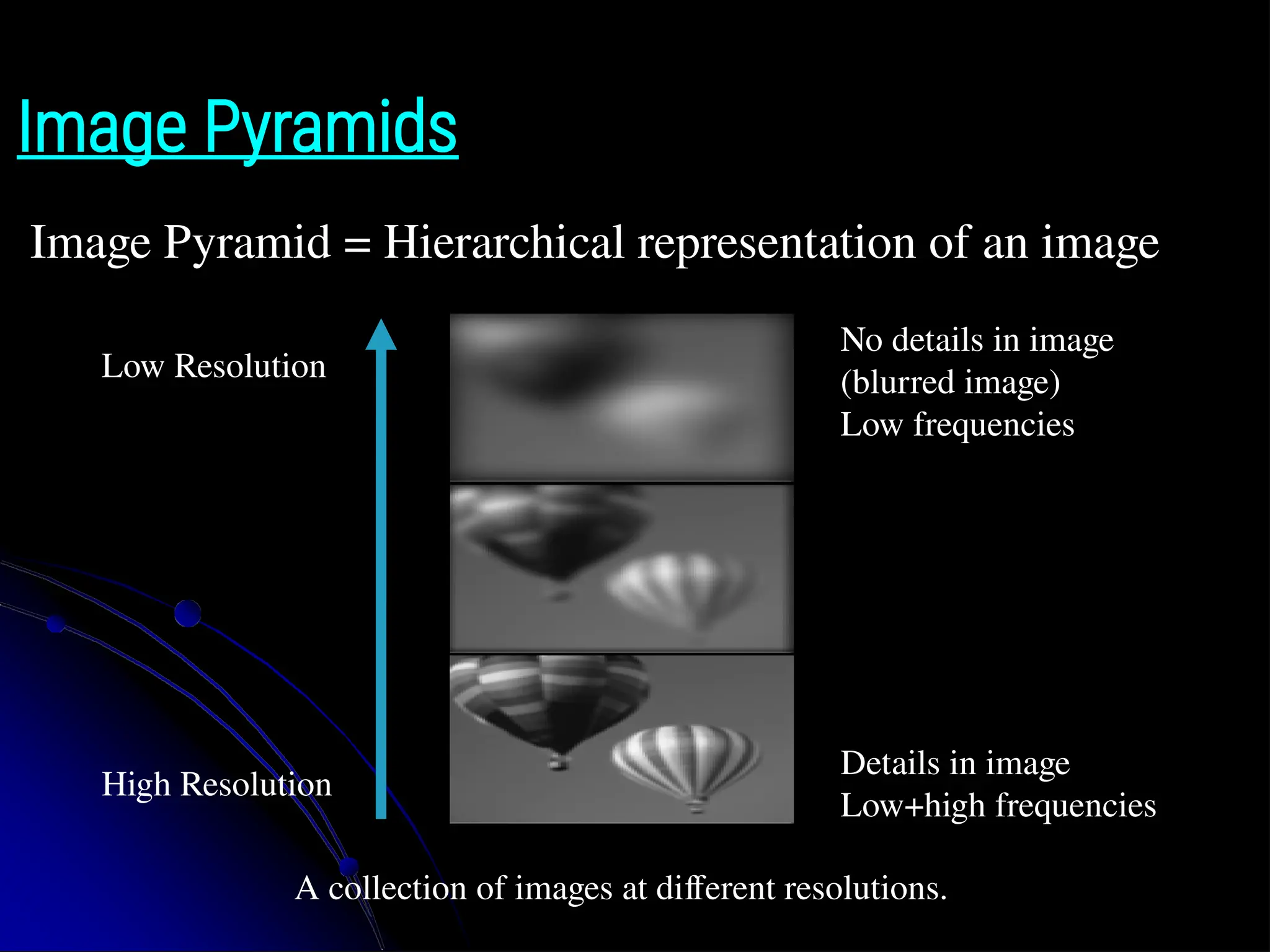
Image Pyramids Image Pyramid= Hierarchical representation of an image Low Resolution High Resolution No details in image (blurred image) Low frequencies Details in image Low+high frequencies A collection of images at different resolutions.
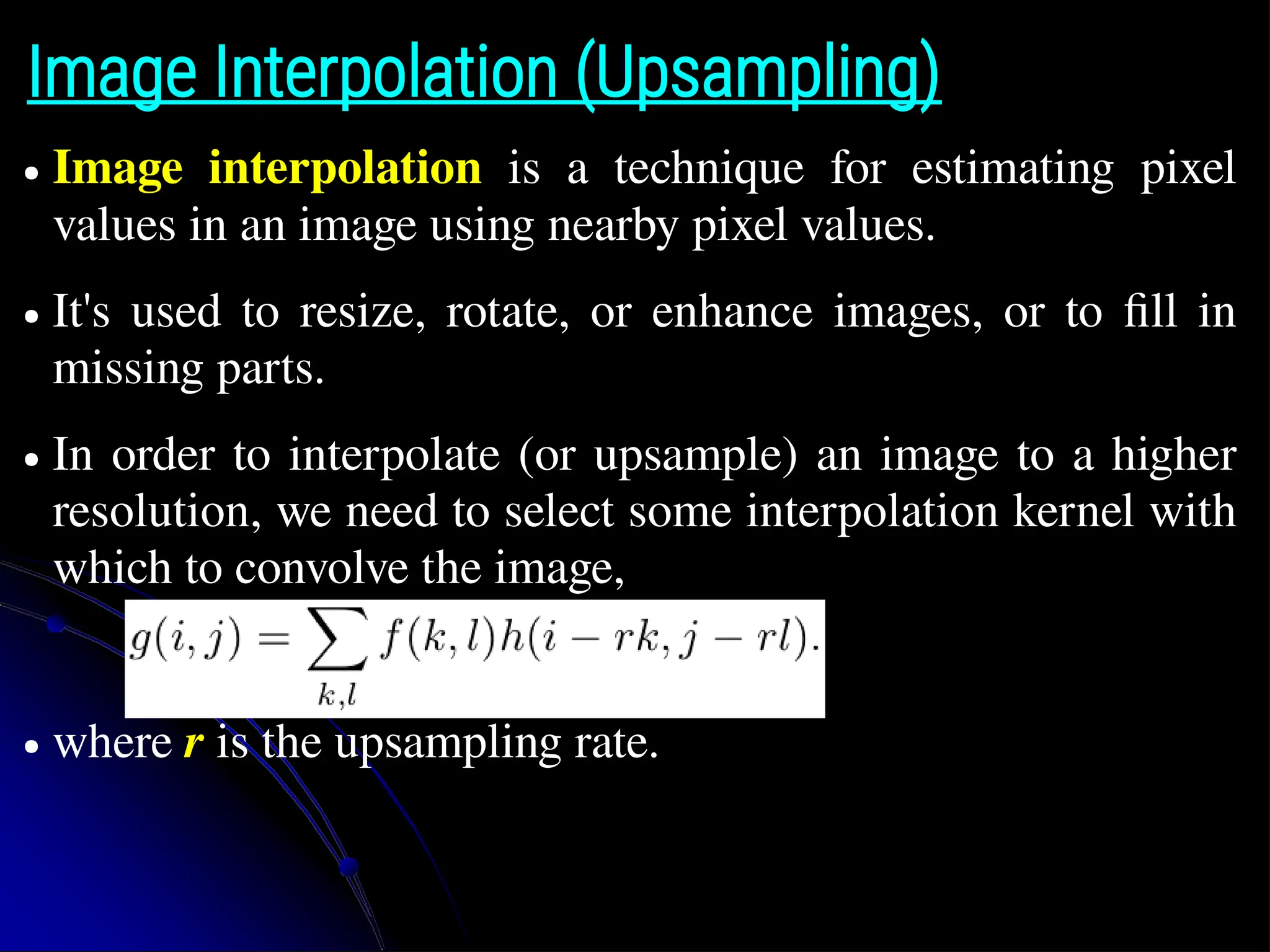
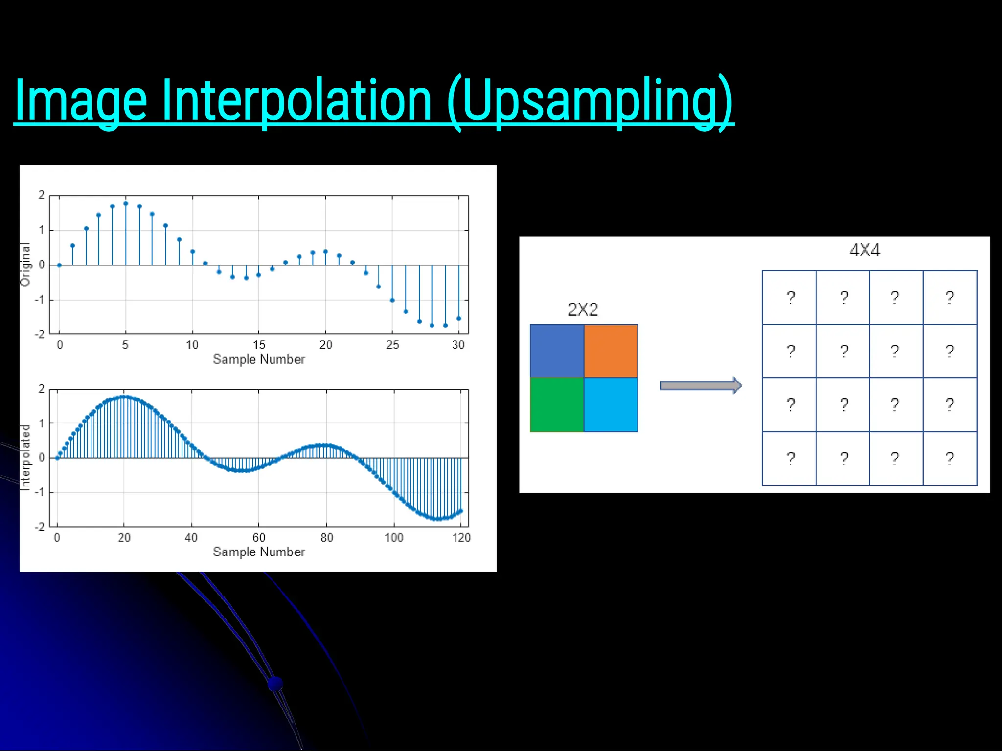
Image Interpolation (Upsampling) ●Image interpolation is a technique for estimating pixel values in an image using nearby pixel values. ● It's used to resize, rotate, or enhance images, or to fill in missing parts. ● In order to interpolate (or upsample) an image to a higher resolution, we need to select some interpolation kernel with which to convolve the image, ● where r is the upsampling rate.
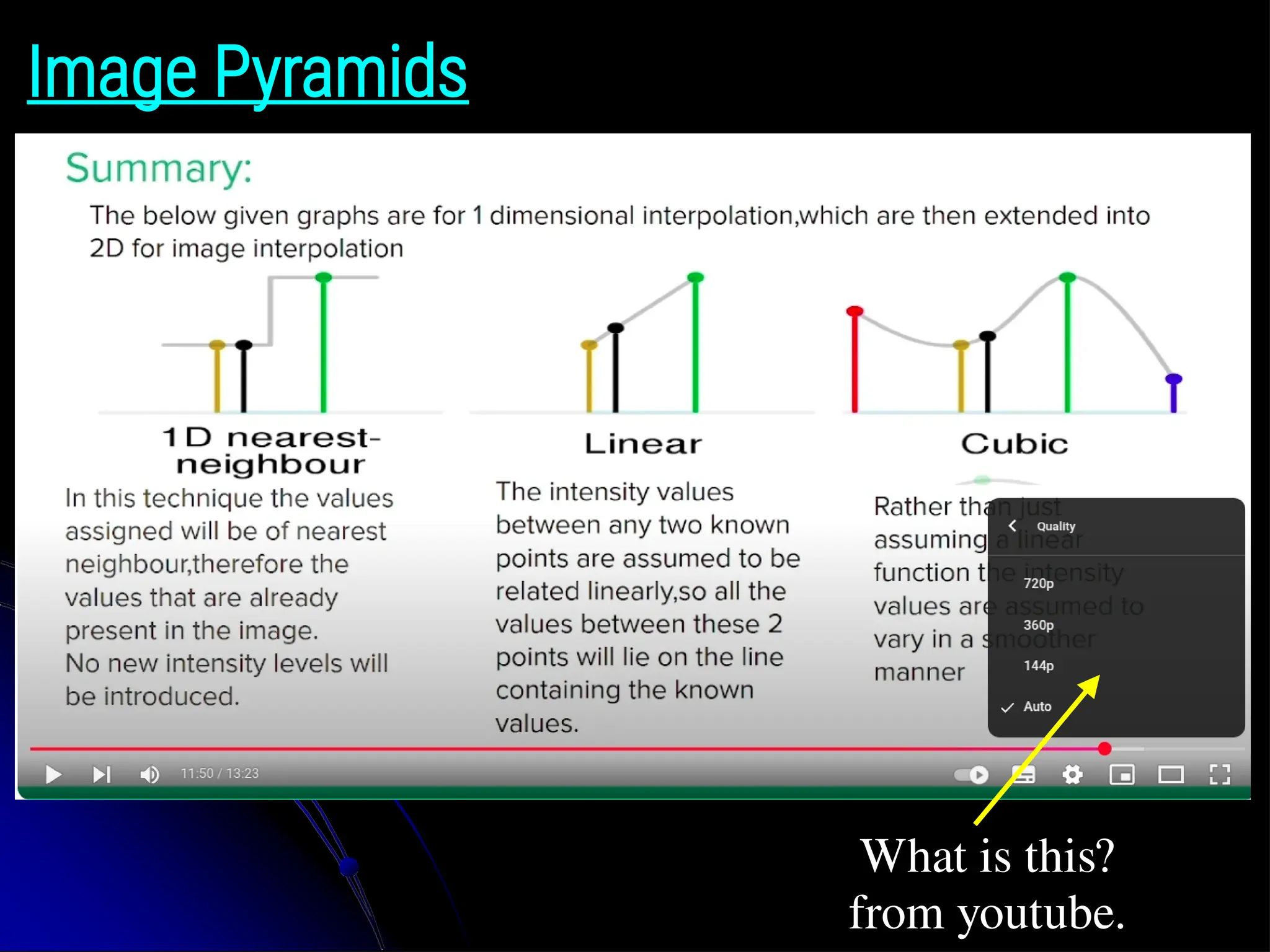
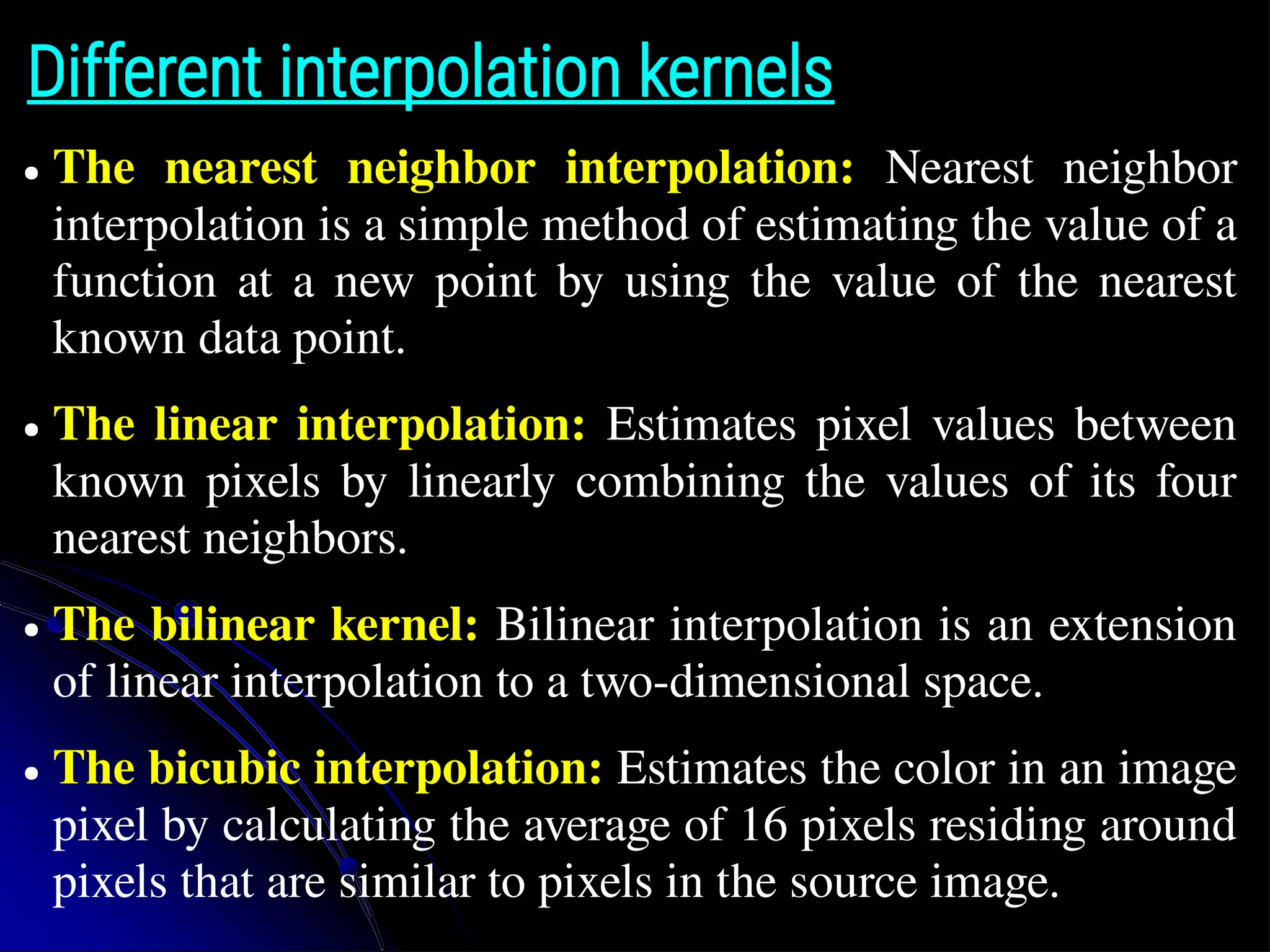
Different interpolation kernels ●The nearest neighbor interpolation: Nearest neighbor interpolation is a simple method of estimating the value of a function at a new point by using the value of the nearest known data point. ● The linear interpolation: Estimates pixel values between known pixels by linearly combining the values of its four nearest neighbors. ● The bilinear kernel: Bilinear interpolation is an extension of linear interpolation to a two-dimensional space. ● The bicubic interpolation: Estimates the color in an image pixel by calculating the average of 16 pixels residing around pixels that are similar to pixels in the source image.
63.
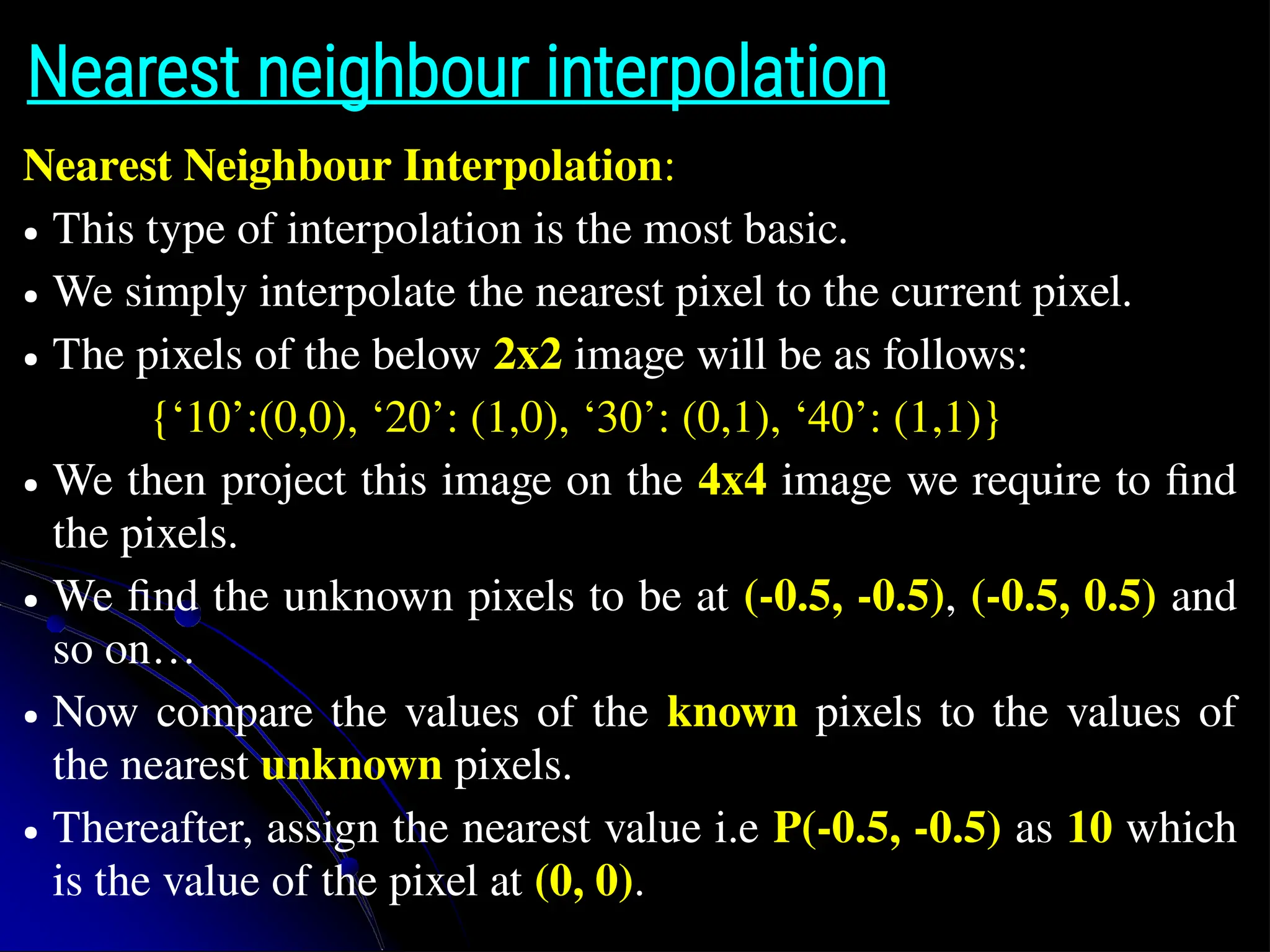
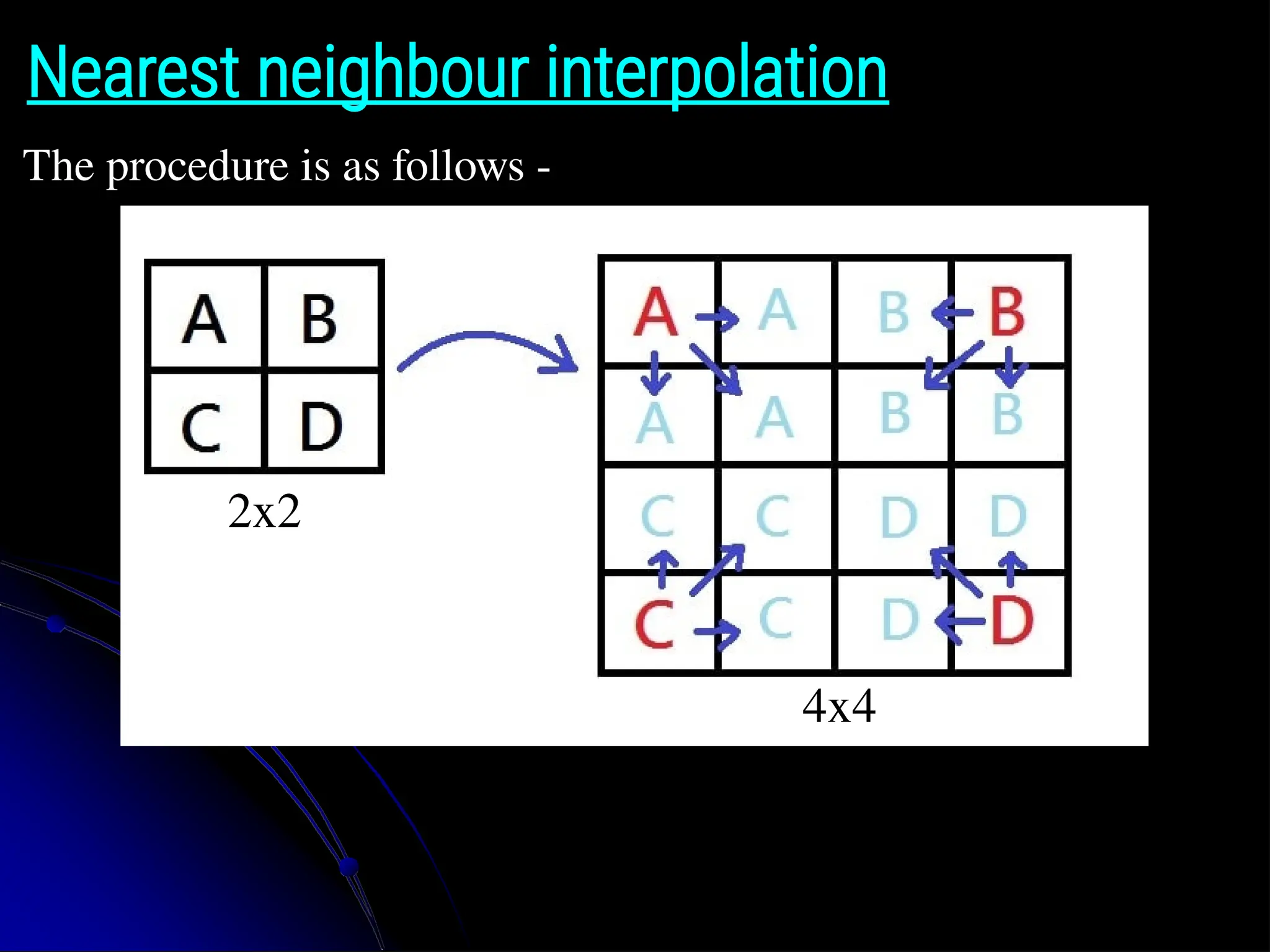
Nearest neighbour interpolation NearestNeighbour Interpolation: ● This type of interpolation is the most basic. ● We simply interpolate the nearest pixel to the current pixel. ● The pixels of the below 2x2 image will be as follows: {‘10’:(0,0), ‘20’: (1,0), ‘30’: (0,1), ‘40’: (1,1)} ● We then project this image on the 4x4 image we require to find the pixels. ● We find the unknown pixels to be at (-0.5, -0.5), (-0.5, 0.5) and so on… ● Now compare the values of the known pixels to the values of the nearest unknown pixels. ● Thereafter, assign the nearest value i.e P(-0.5, -0.5) as 10 which is the value of the pixel at (0, 0).
64.
The procedure isas follows - Nearest neighbour interpolation 2x2 4x4
65.
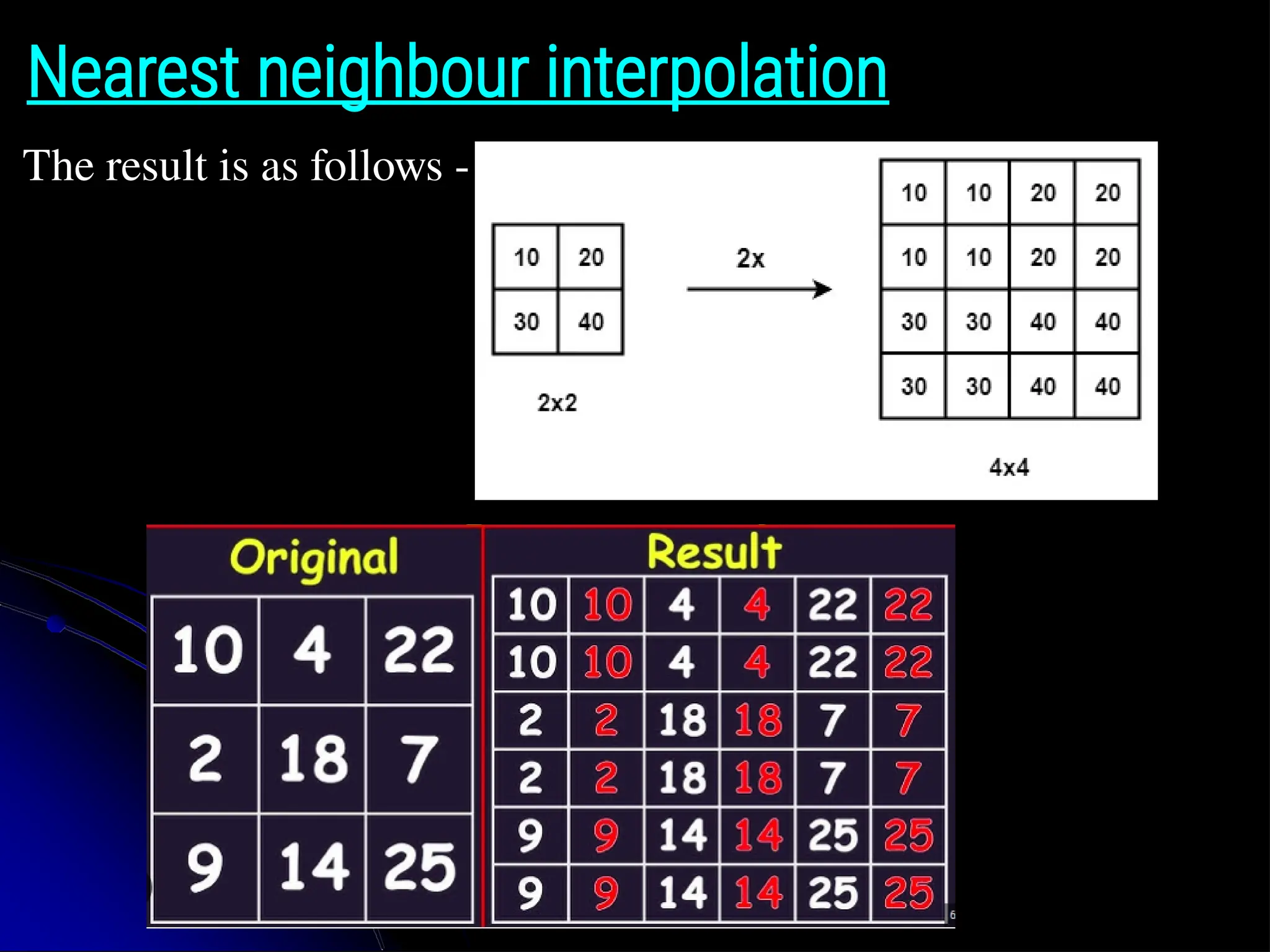
The result isas follows - Nearest neighbour interpolation
66.
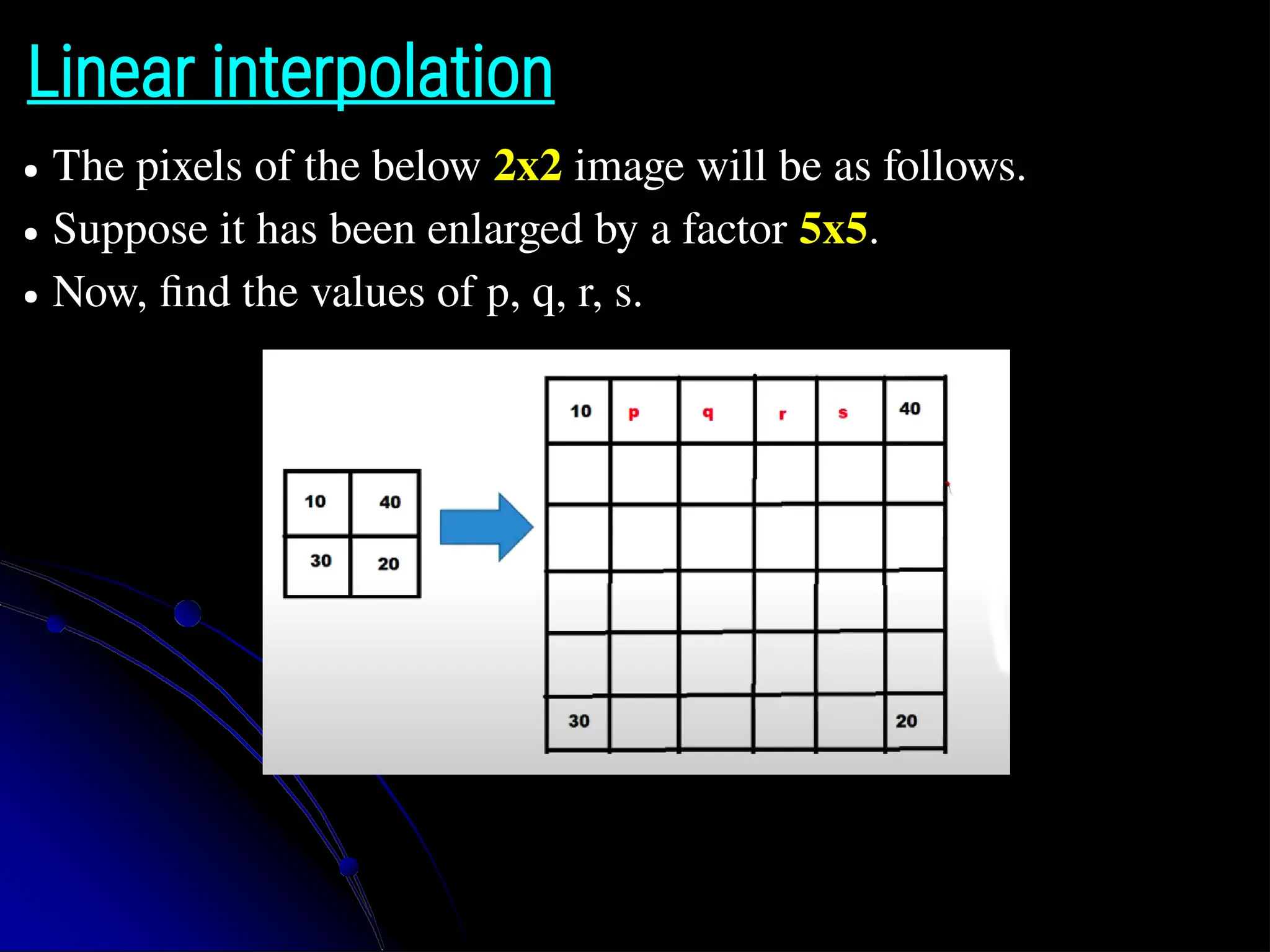
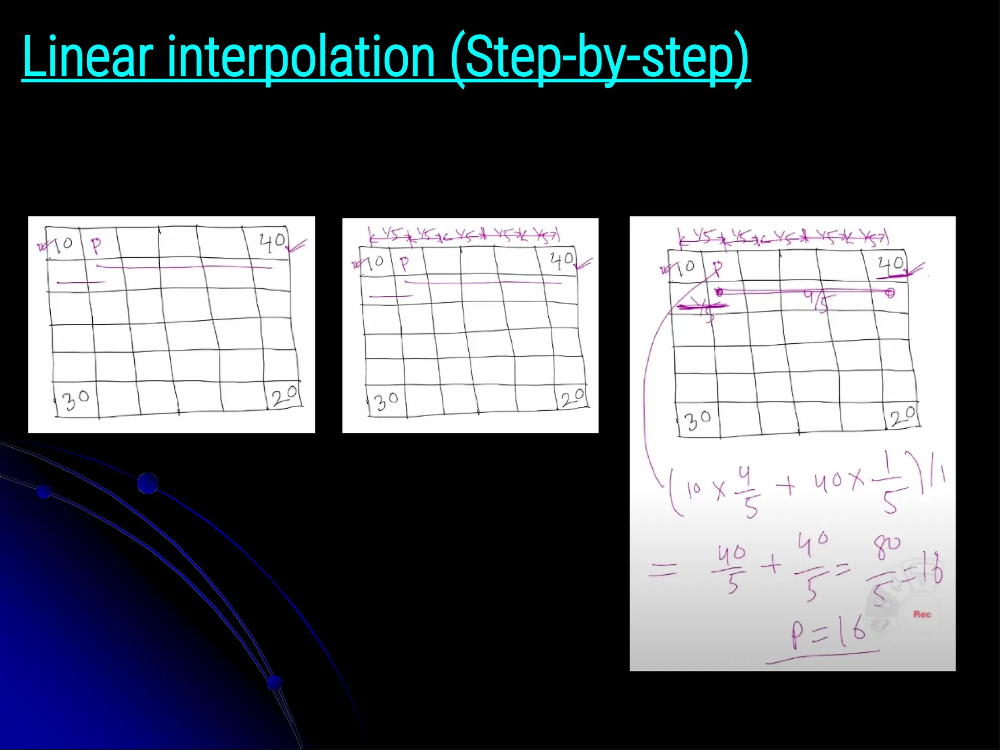
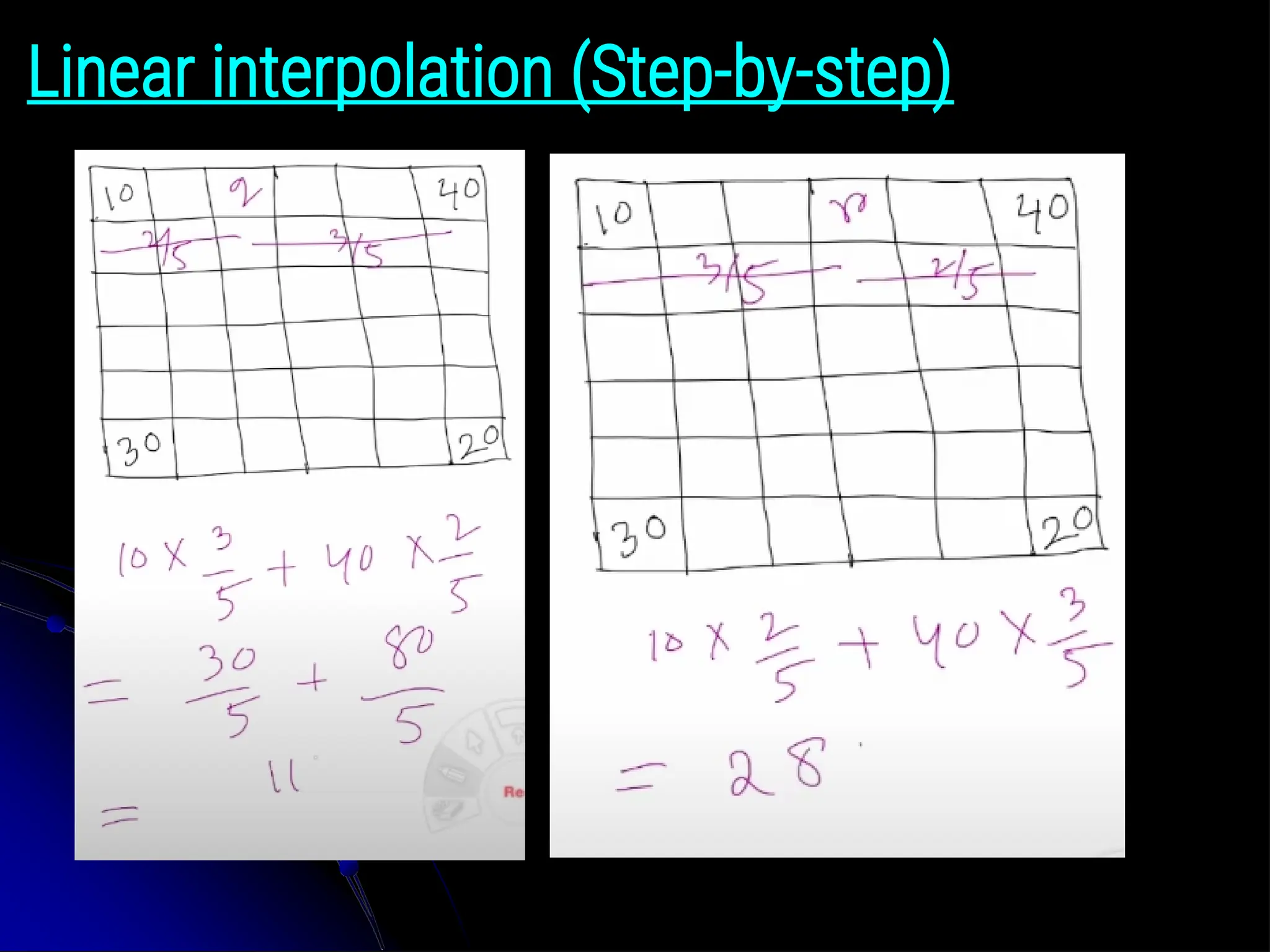
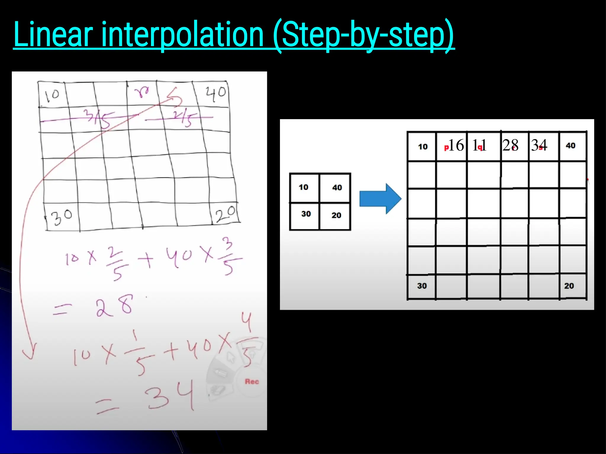
Linear interpolation ● Thepixels of the below 2x2 image will be as follows. ● Suppose it has been enlarged by a factor 5x5. ● Now, find the values of p, q, r, s.
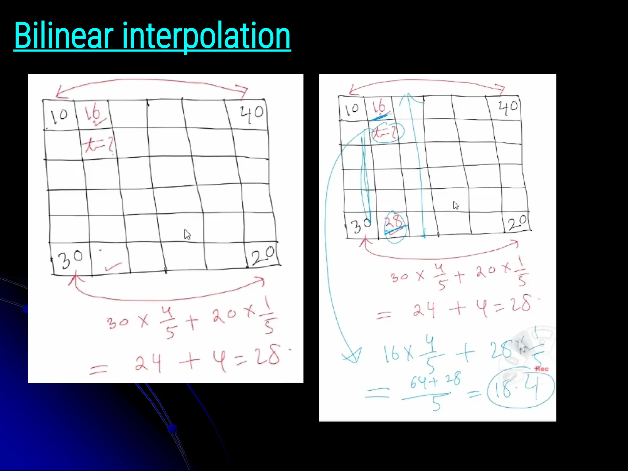
Bilinear interpolation ● Inbilinear interpolation we take the values of four nearest known neighbours (2x2 neighbourhood) of unknown pixels and then take the average of these values to assign the unknown pixel. ● Let’s first understand how this would work on a simple example. Suppose we take a random point say (0.75, 0.25) which is in the middle of four points – (0,0), (0,1), (1,0), (1,1). ● We first find the values at points A(0.75, 0) and B(0.75, 1) using linear interpolation. ● We then find the value of the pixel required (0.75, 0.25) using linear interpolation on points A and B.
71.
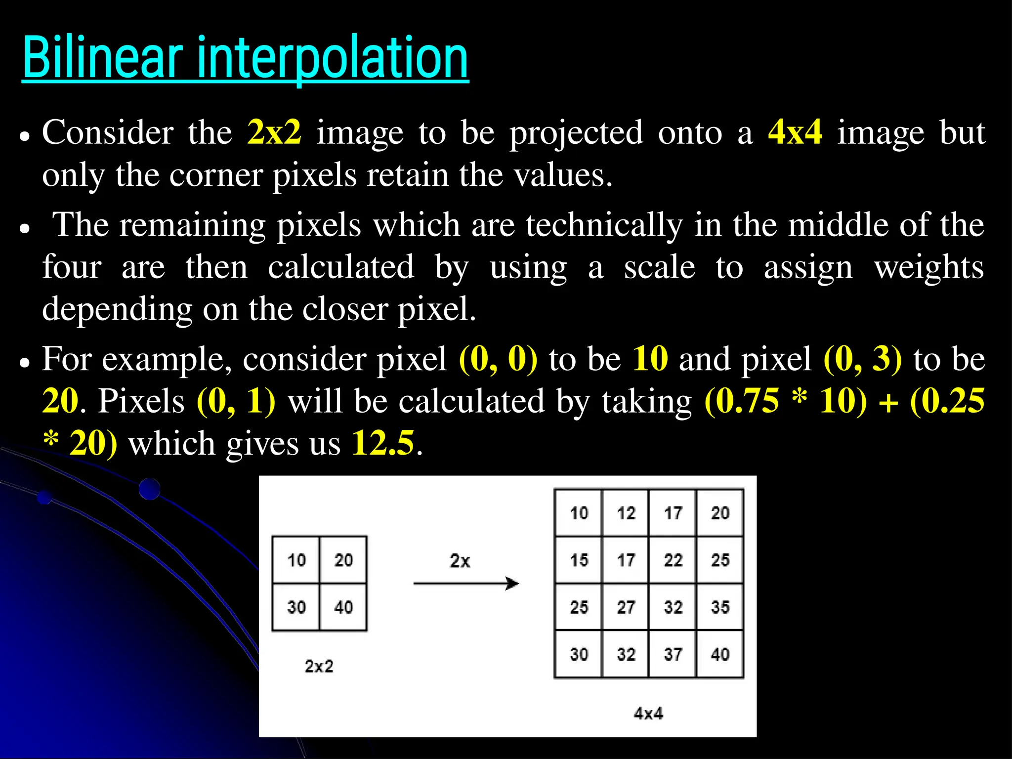
Bilinear interpolation ● Considerthe 2x2 image to be projected onto a 4x4 image but only the corner pixels retain the values. ● The remaining pixels which are technically in the middle of the four are then calculated by using a scale to assign weights depending on the closer pixel. ● For example, consider pixel (0, 0) to be 10 and pixel (0, 3) to be 20. Pixels (0, 1) will be calculated by taking (0.75 * 10) + (0.25 * 20) which gives us 12.5.
72.
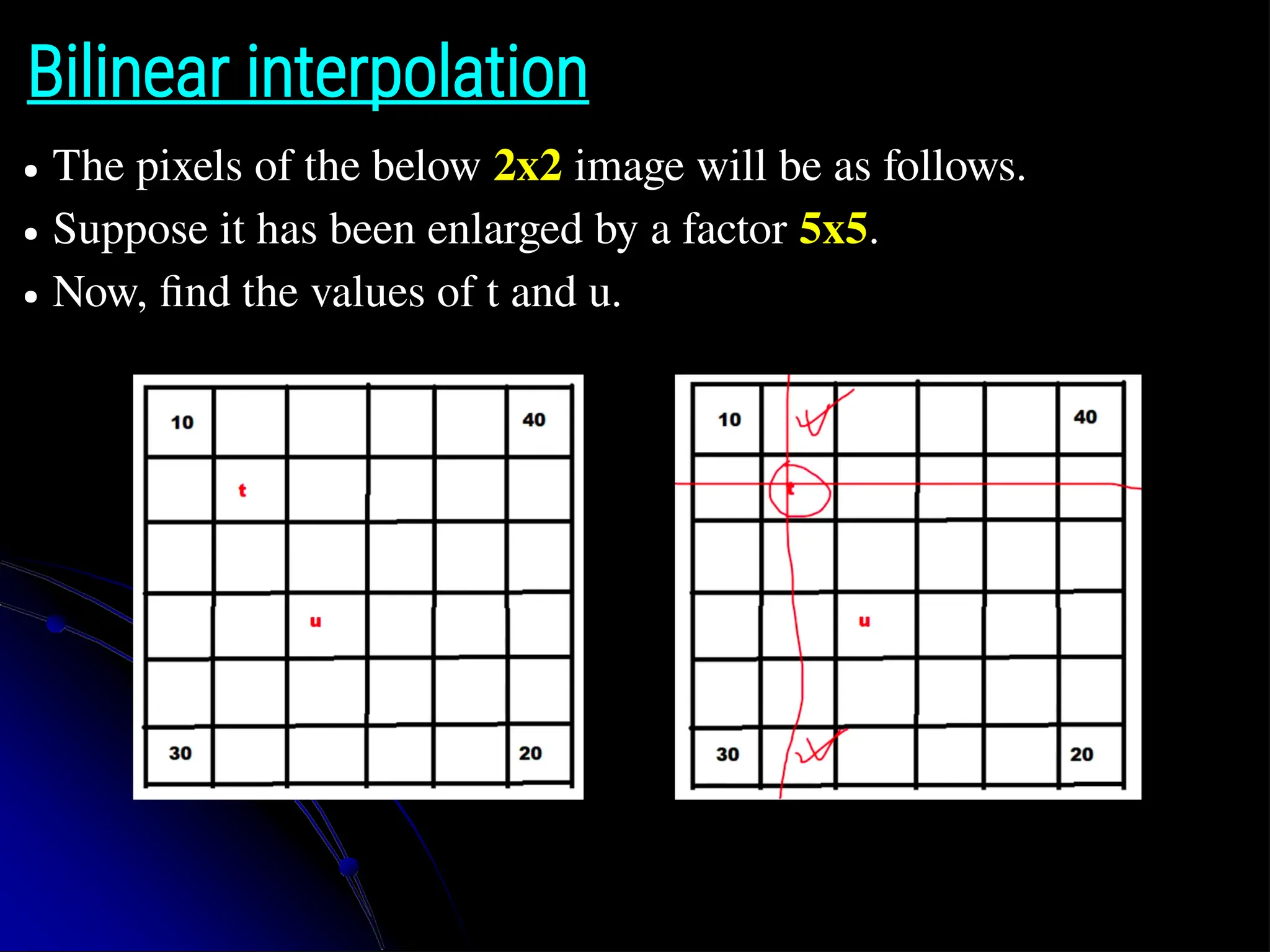
Bilinear interpolation ● Thepixels of the below 2x2 image will be as follows. ● Suppose it has been enlarged by a factor 5x5. ● Now, find the values of t and u.
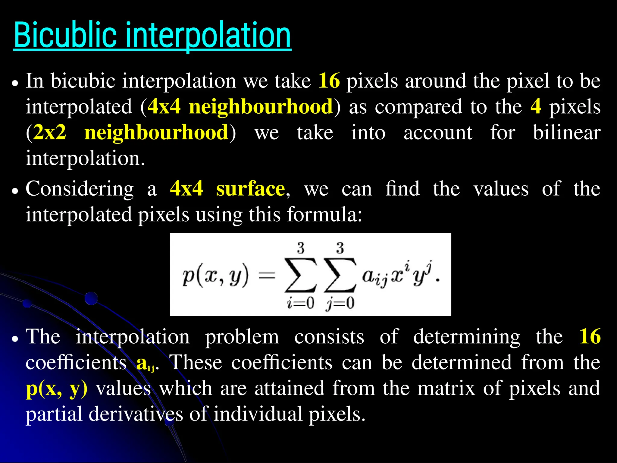
Bicublic interpolation ● Inbicubic interpolation we take 16 pixels around the pixel to be interpolated (4x4 neighbourhood) as compared to the 4 pixels (2x2 neighbourhood) we take into account for bilinear interpolation. ● Considering a 4x4 surface, we can find the values of the interpolated pixels using this formula: ● The interpolation problem consists of determining the 16 coefficients aᵢⱼ. These coefficients can be determined from the p(x, y) values which are attained from the matrix of pixels and partial derivatives of individual pixels.
75.
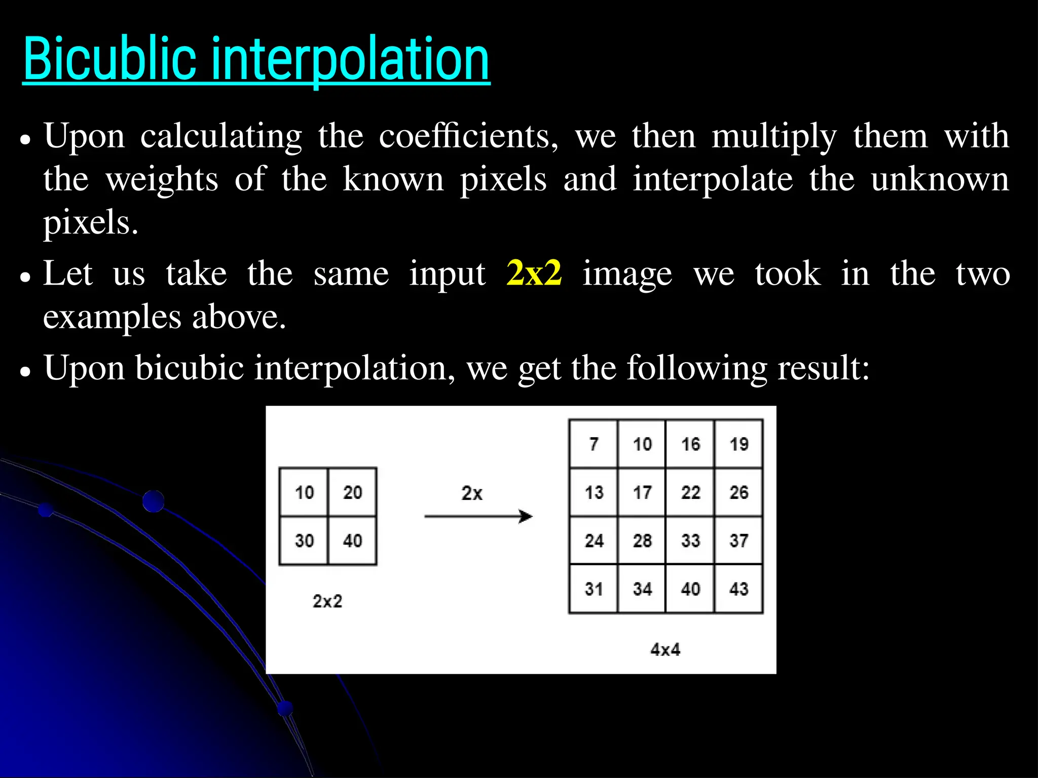
Bicublic interpolation ● Uponcalculating the coefficients, we then multiply them with the weights of the known pixels and interpolate the unknown pixels. ● Let us take the same input 2x2 image we took in the two examples above. ● Upon bicubic interpolation, we get the following result:
76.
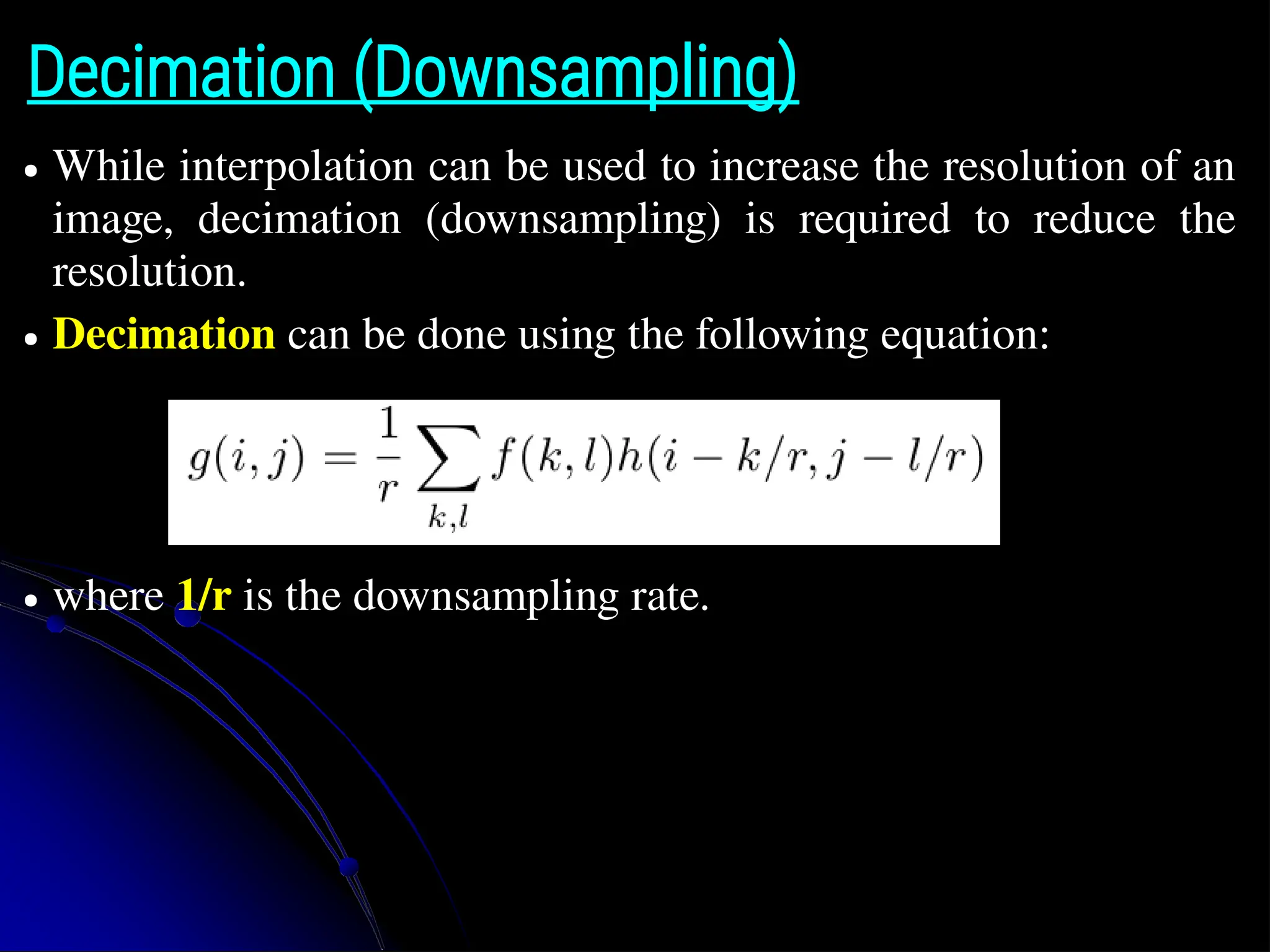
Decimation (Downsampling) ● Whileinterpolation can be used to increase the resolution of an image, decimation (downsampling) is required to reduce the resolution. ● Decimation can be done using the following equation: ● where 1/r is the downsampling rate.
77.
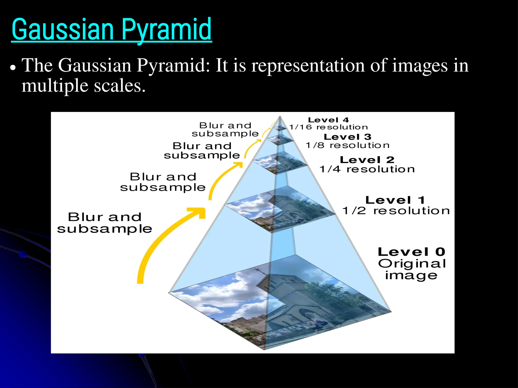
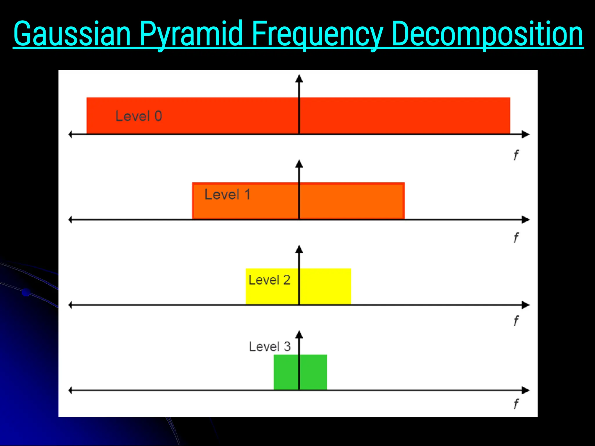
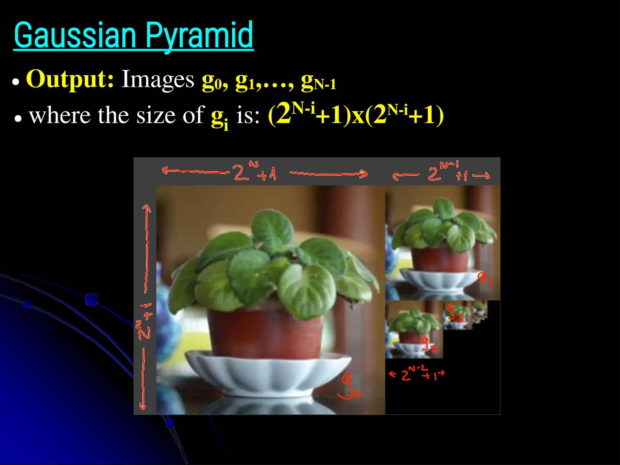
Gaussian Pyramid ● TheGaussian Pyramid: It is representation of images in multiple scales.
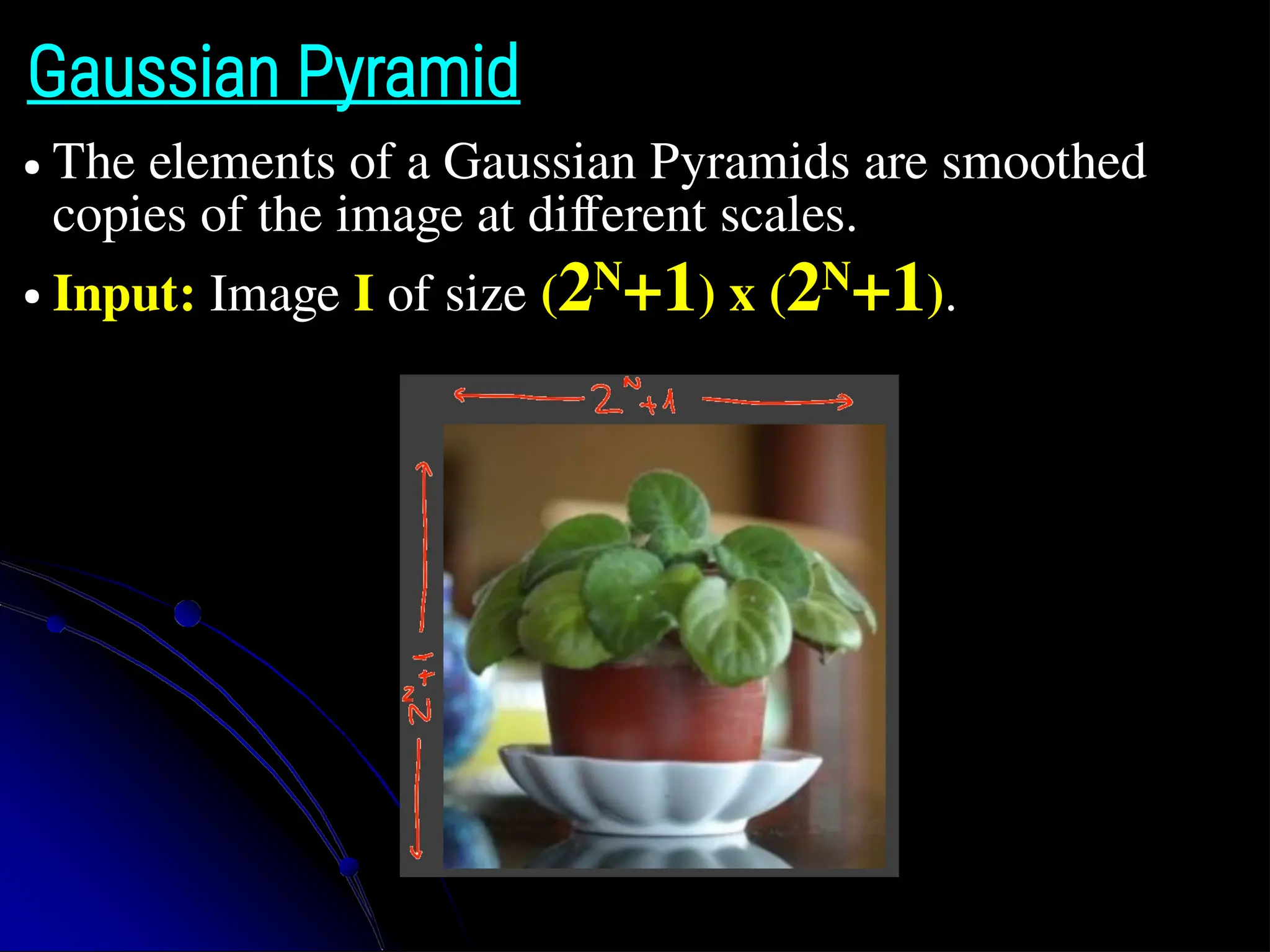
Gaussian Pyramid ● Theelements of a Gaussian Pyramids are smoothed copies of the image at different scales. ● Input: Image I of size (2N +1) x (2N +1).
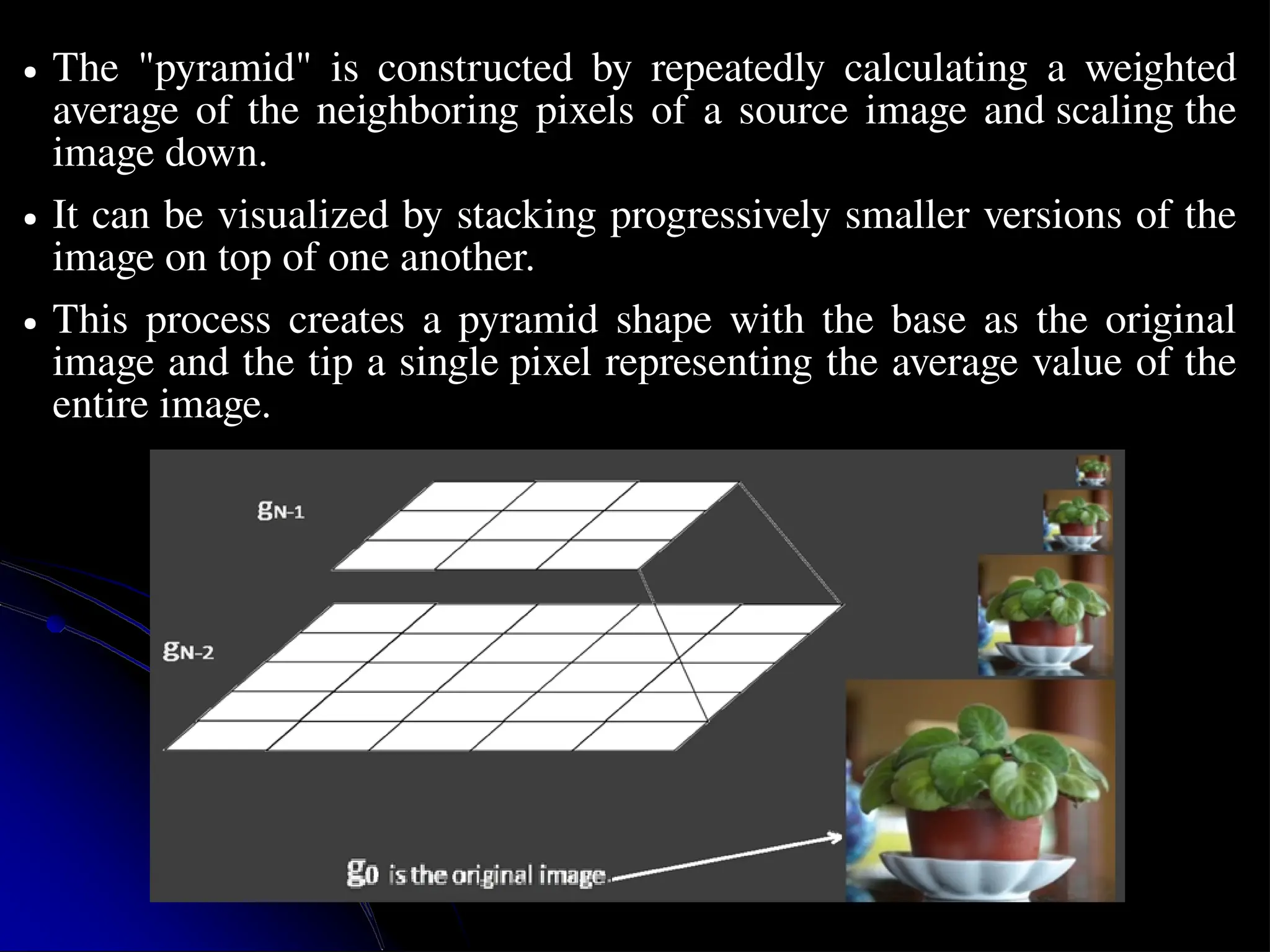
● The "pyramid"is constructed by repeatedly calculating a weighted average of the neighboring pixels of a source image and scaling the image down. ● It can be visualized by stacking progressively smaller versions of the image on top of one another. ● This process creates a pyramid shape with the base as the original image and the tip a single pixel representing the average value of the entire image.
82.
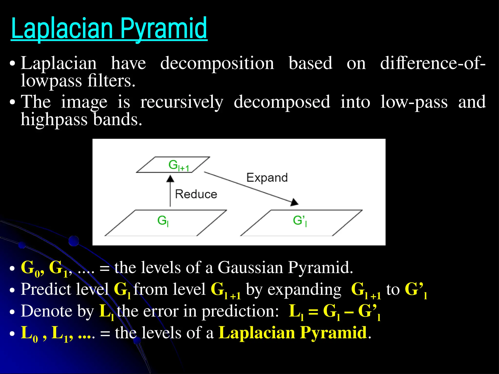
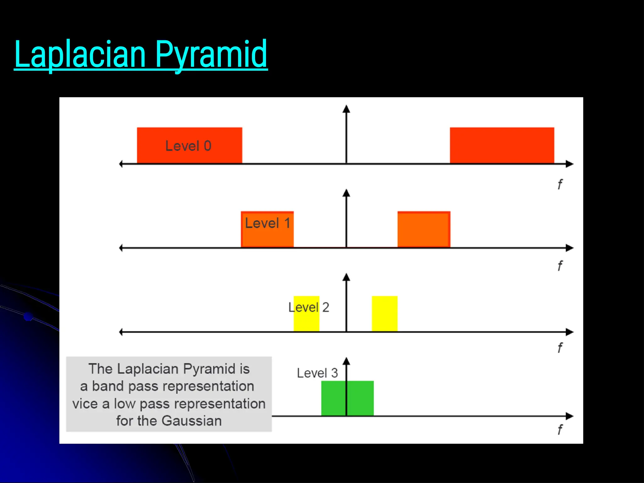
Laplacian Pyramid ● Laplacianhave decomposition based on difference-of- lowpass filters. ● The image is recursively decomposed into low-pass and highpass bands. ● G0, G1, .... = the levels of a Gaussian Pyramid. ● Predict level Gl from level Gl +1 by expanding Gl +1 to G’l ● Denote by Ll the error in prediction: Ll = Gl – G’l ● L0 , L1, .... = the levels of a Laplacian Pyramid.
83.
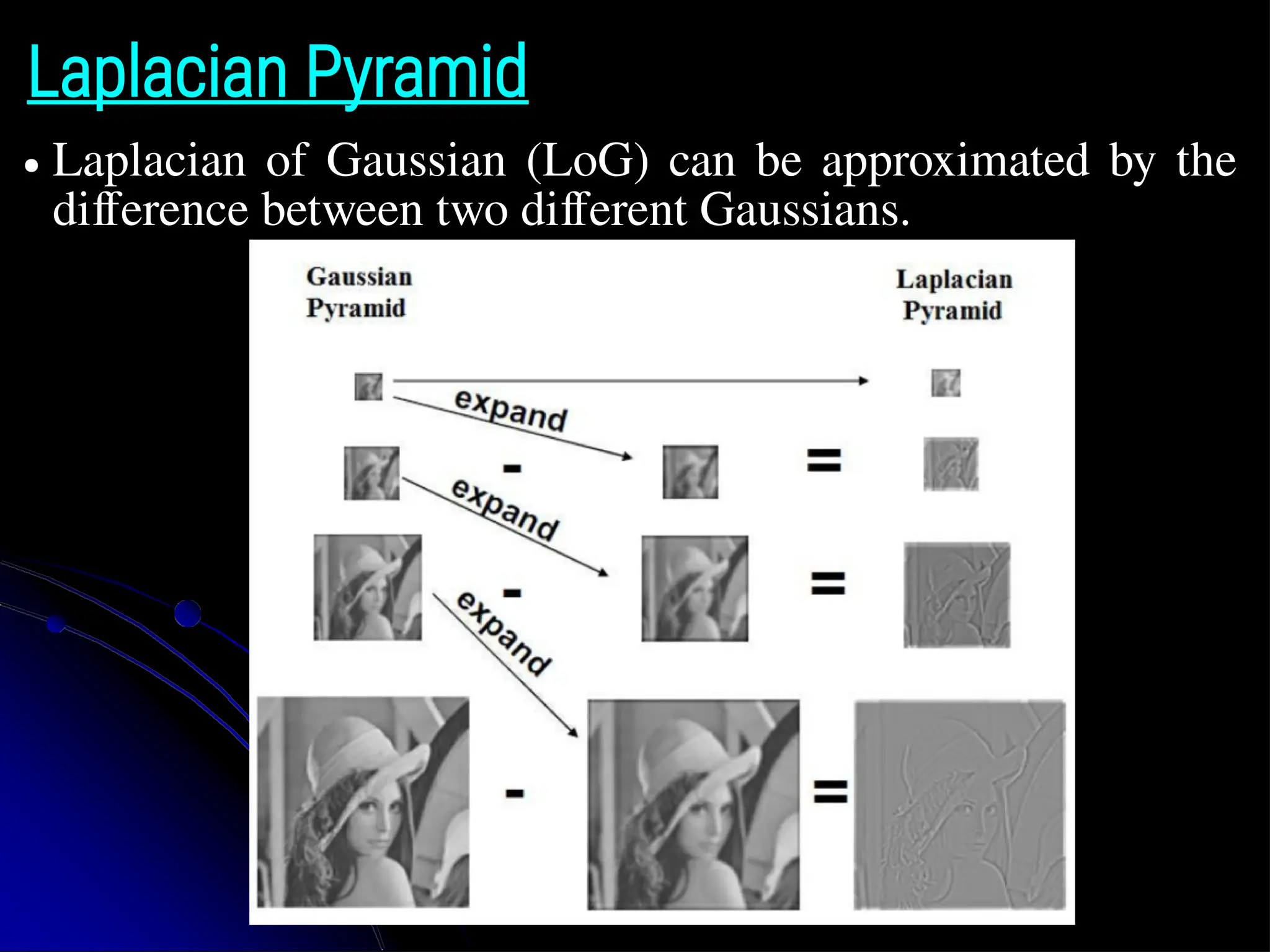
Laplacian Pyramid ● Laplacianof Gaussian (LoG) can be approximated by the difference between two different Gaussians.
84.
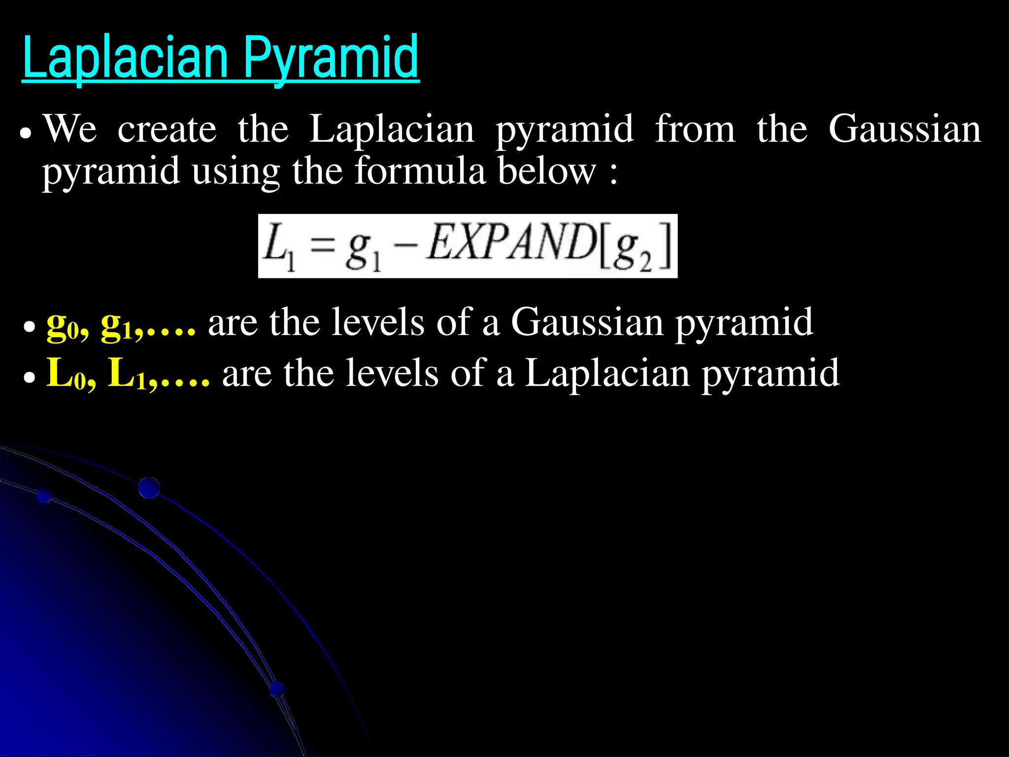
Laplacian Pyramid ● Wecreate the Laplacian pyramid from the Gaussian pyramid using the formula below : ● g0, g1,…. are the levels of a Gaussian pyramid ● L0, L1,…. are the levels of a Laplacian pyramid
Wavelet Transforms ● FourierTransforms are used extensively in computer vision applications, but some people use wavelet decompositions as an alternative. ● Wavelets can solve and model complex signal processing problems. ● Wavelets are filters that localize a signal in both time and frequency and are defined over a hierarchy of scales. ● Wavelets provide a smooth way to decompose a signal into frequency components without blocking and are closely related to pyramids.
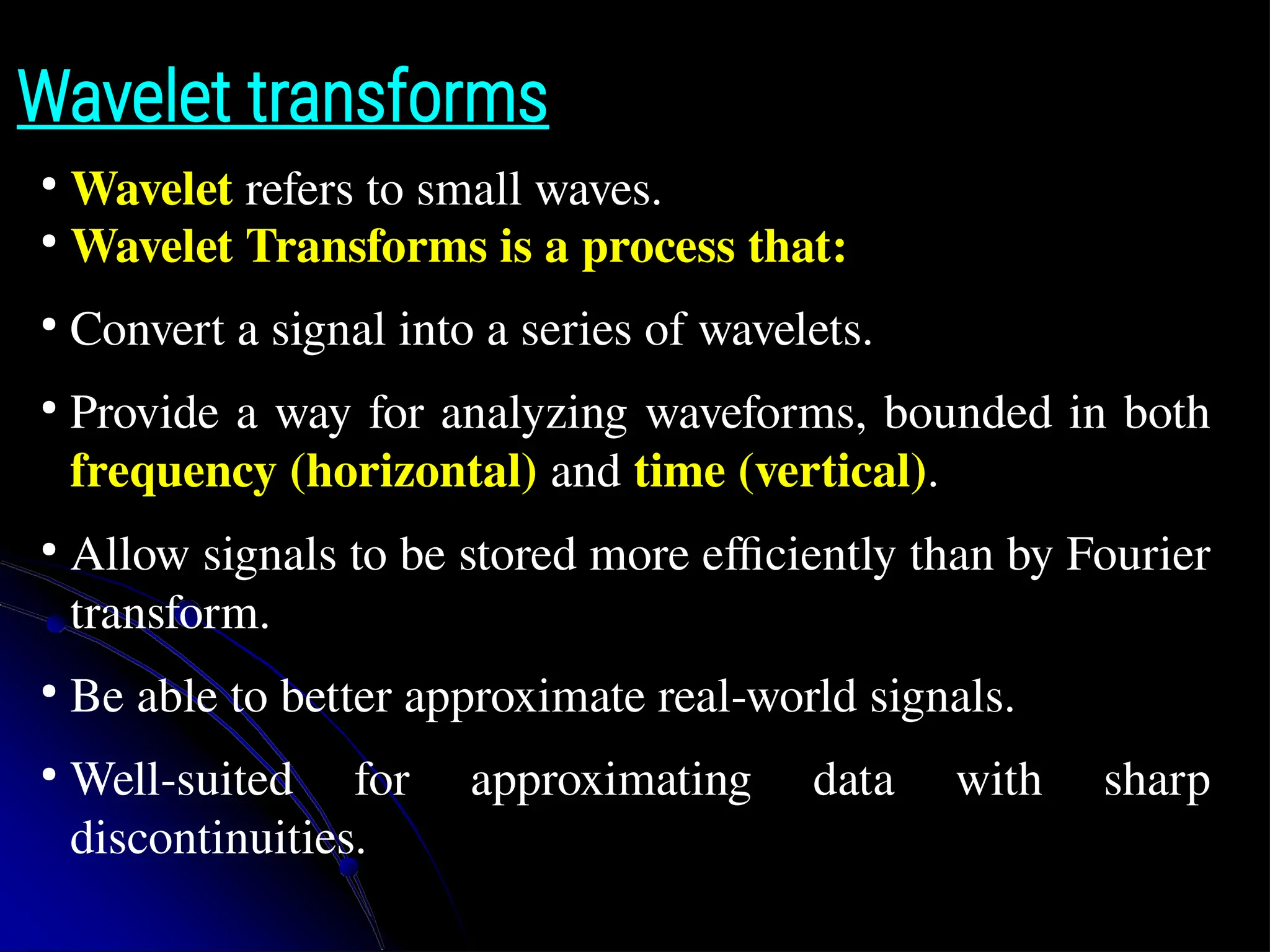
Wavelet transforms ● Wavelet refersto small waves. ● Wavelet Transforms is a process that: ● Convert a signal into a series of wavelets. ● Provide a way for analyzing waveforms, bounded in both frequency (horizontal) and time (vertical). ● Allow signals to be stored more efficiently than by Fourier transform. ● Be able to better approximate real-world signals. ● Well-suited for approximating data with sharp discontinuities.
89.
Principles of wavelettransforms ● Split up the signal into a set of small signals. ● Representing the same signal in different frequency bands. ● Provides different frequency bands at different time intervals. ● This helps in multi-resolution signal analysis.
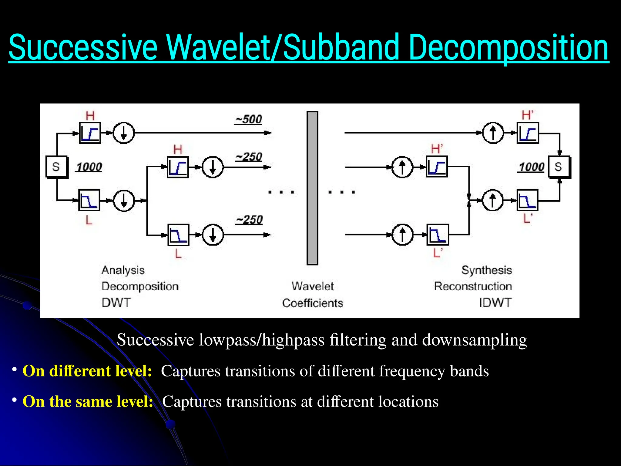
Successive Wavelet/Subband Decomposition Successivelowpass/highpass filtering and downsampling ● On different level: Captures transitions of different frequency bands ● On the same level: Captures transitions at different locations
92.
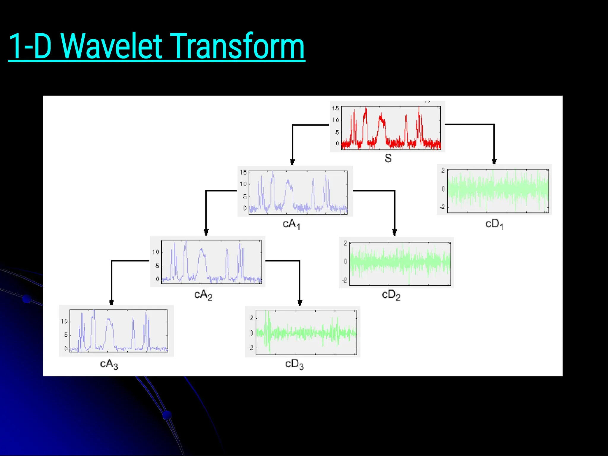
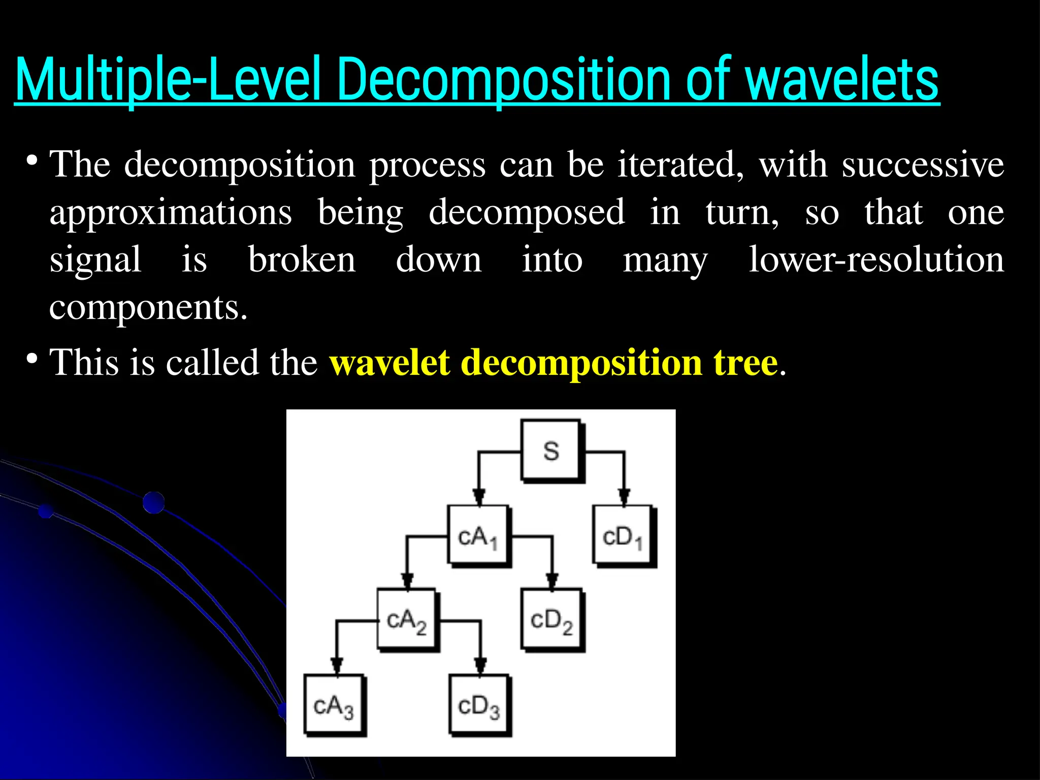
Multiple-Level Decomposition ofwavelets ● The decomposition process can be iterated, with successive approximations being decomposed in turn, so that one signal is broken down into many lower-resolution components. ● This is called the wavelet decomposition tree.
93.
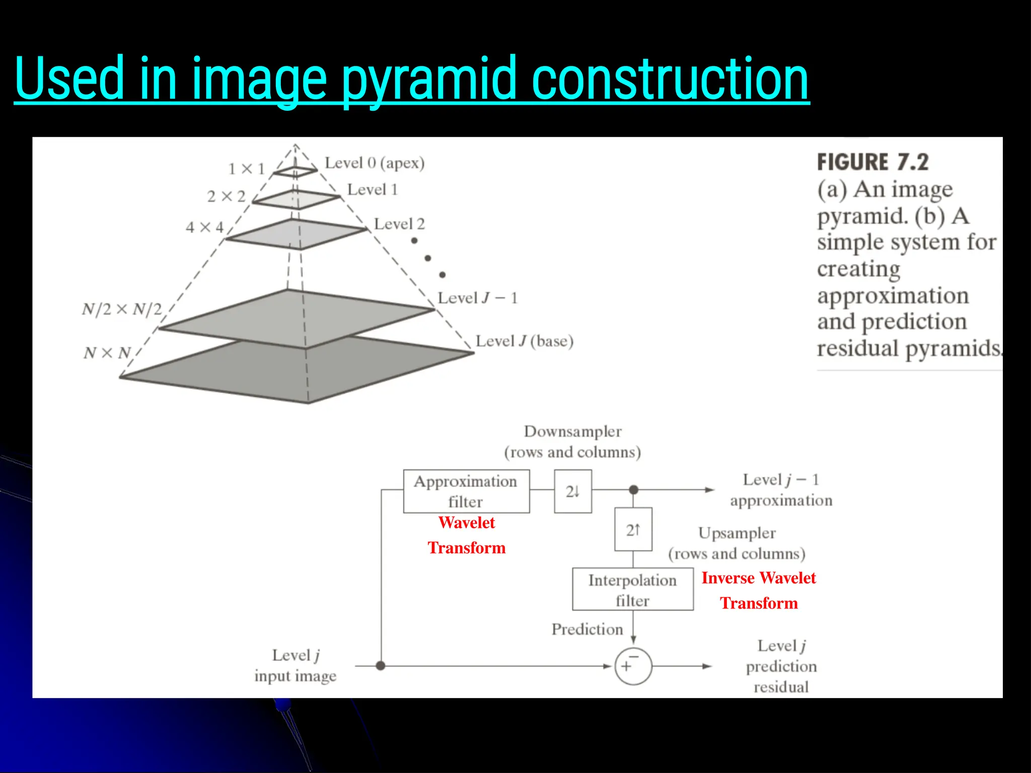
Used in imagepyramid construction Wavelet Transform Inverse Wavelet Transform
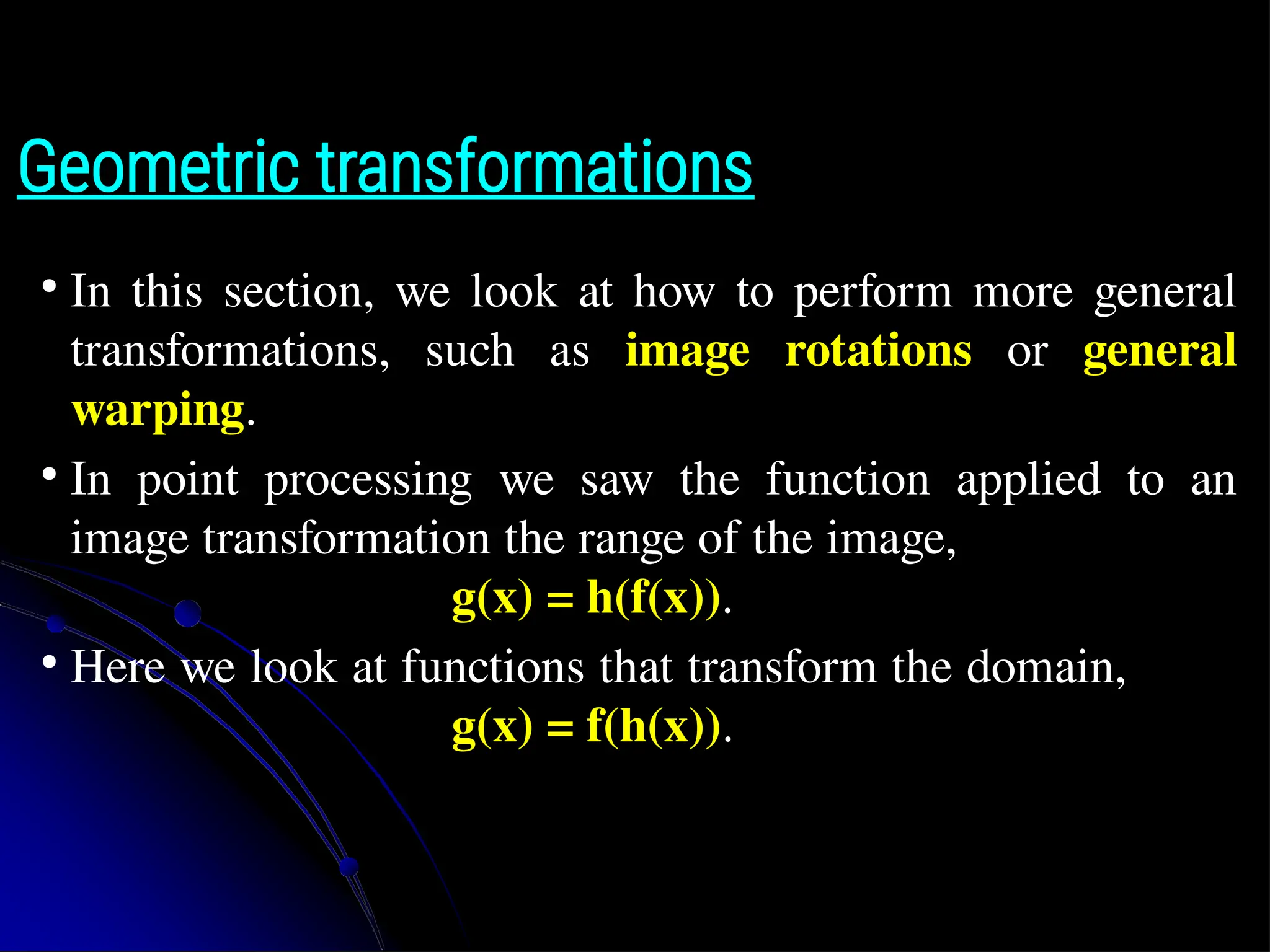
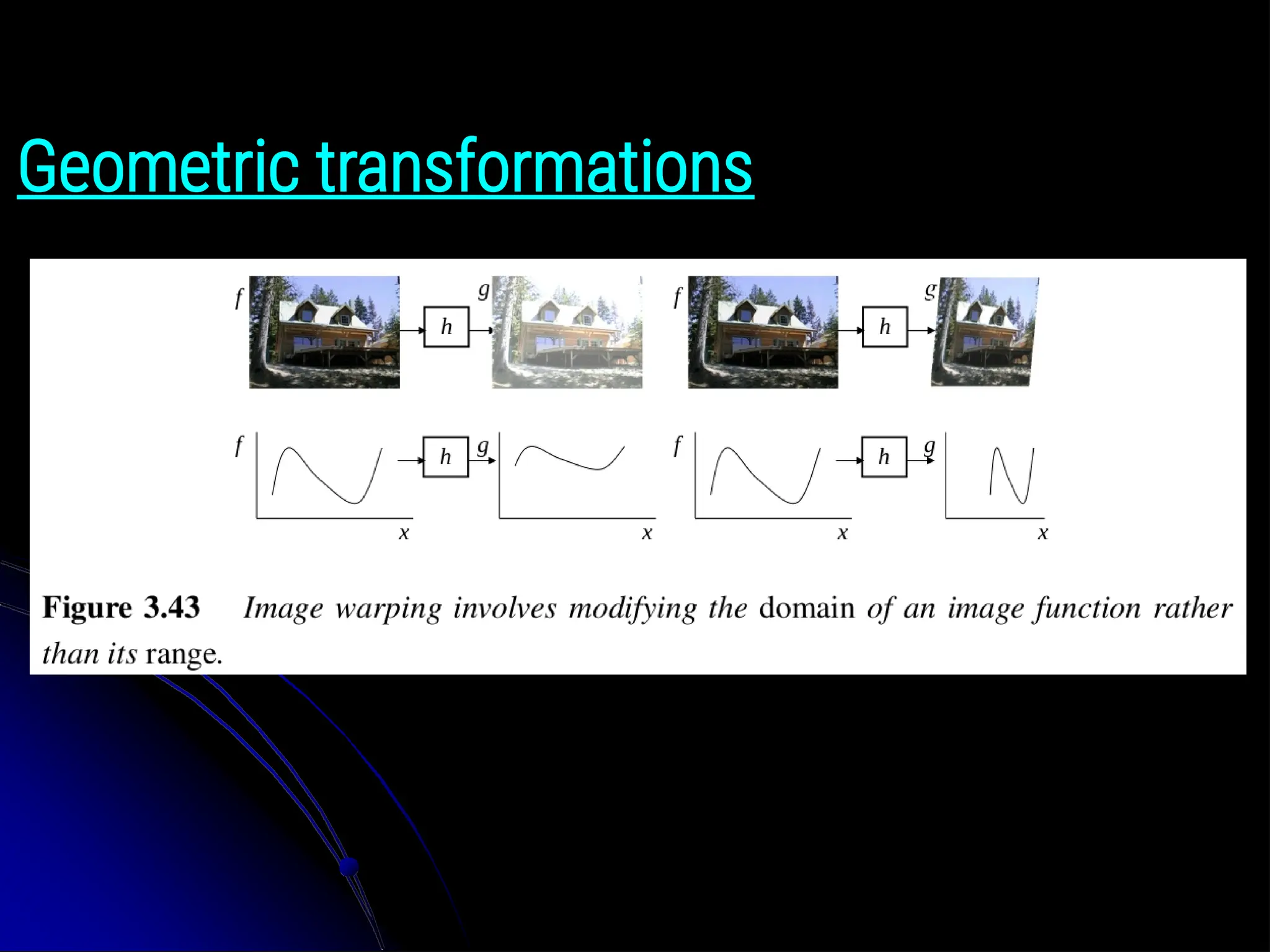
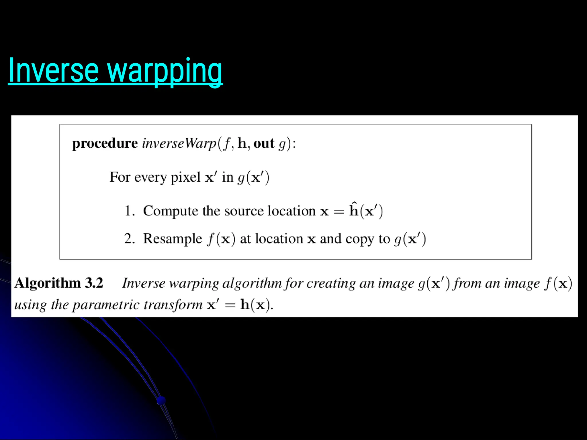
Geometric transformations ● In thissection, we look at how to perform more general transformations, such as image rotations or general warping. ● In point processing we saw the function applied to an image transformation the range of the image, g(x) = h(f(x)). ● Here we look at functions that transform the domain, g(x) = f(h(x)).
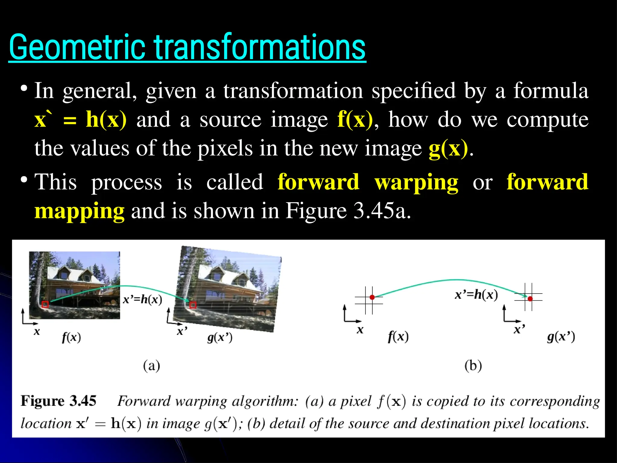
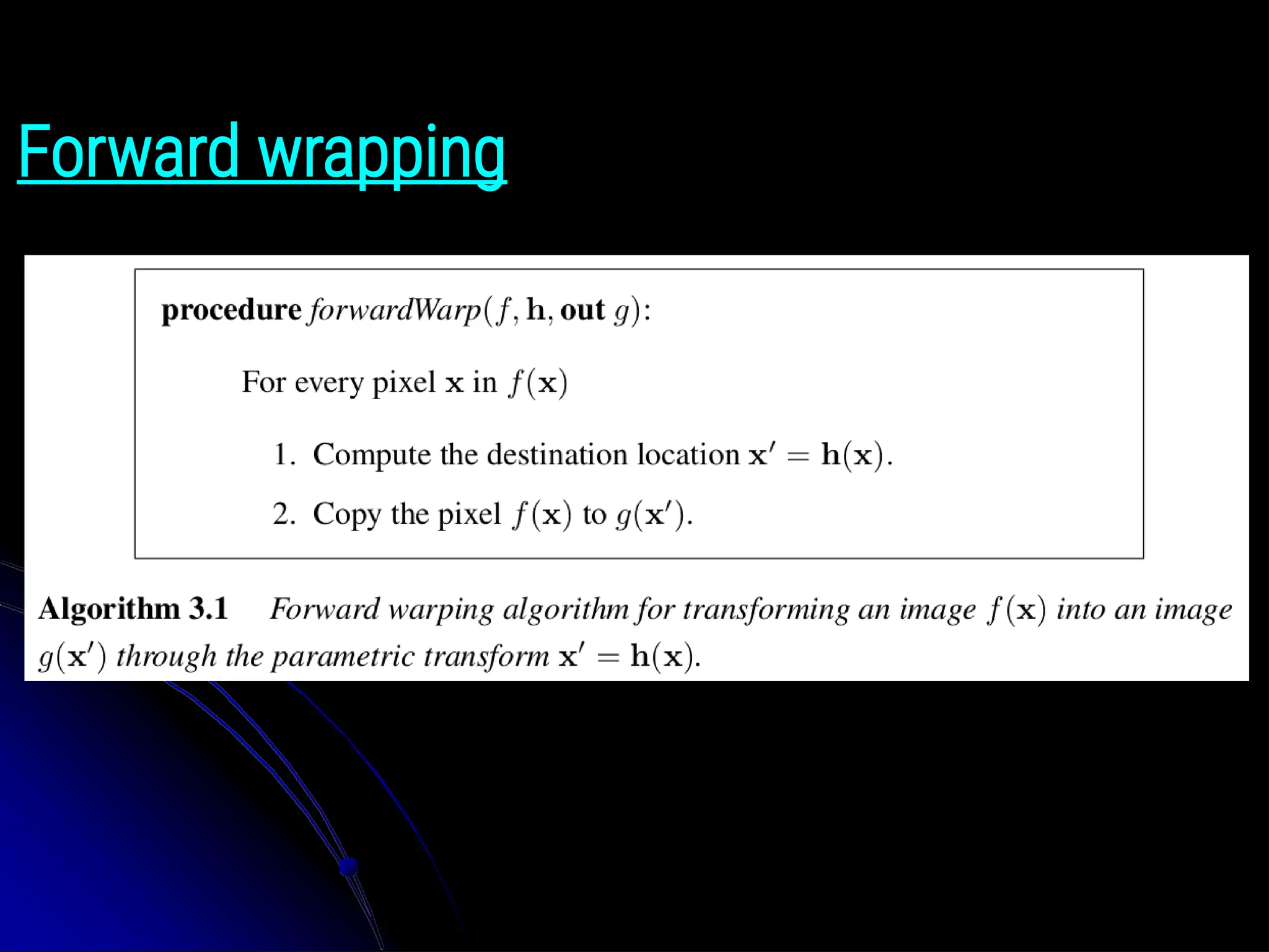
Geometric transformations ● In general,given a transformation specified by a formula x` = h(x) and a source image f(x), how do we compute the values of the pixels in the new image g(x). ● This process is called forward warping or forward mapping and is shown in Figure 3.45a.
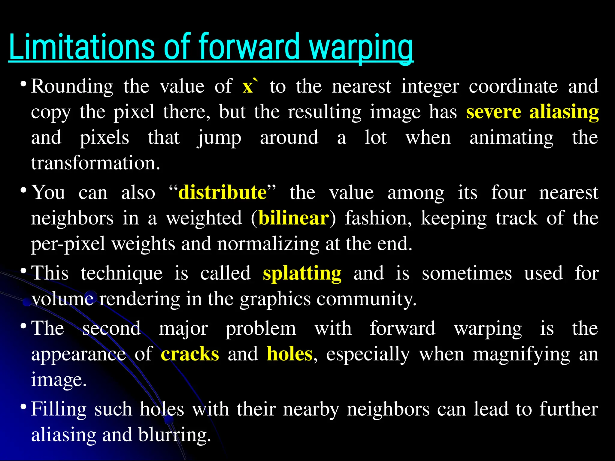
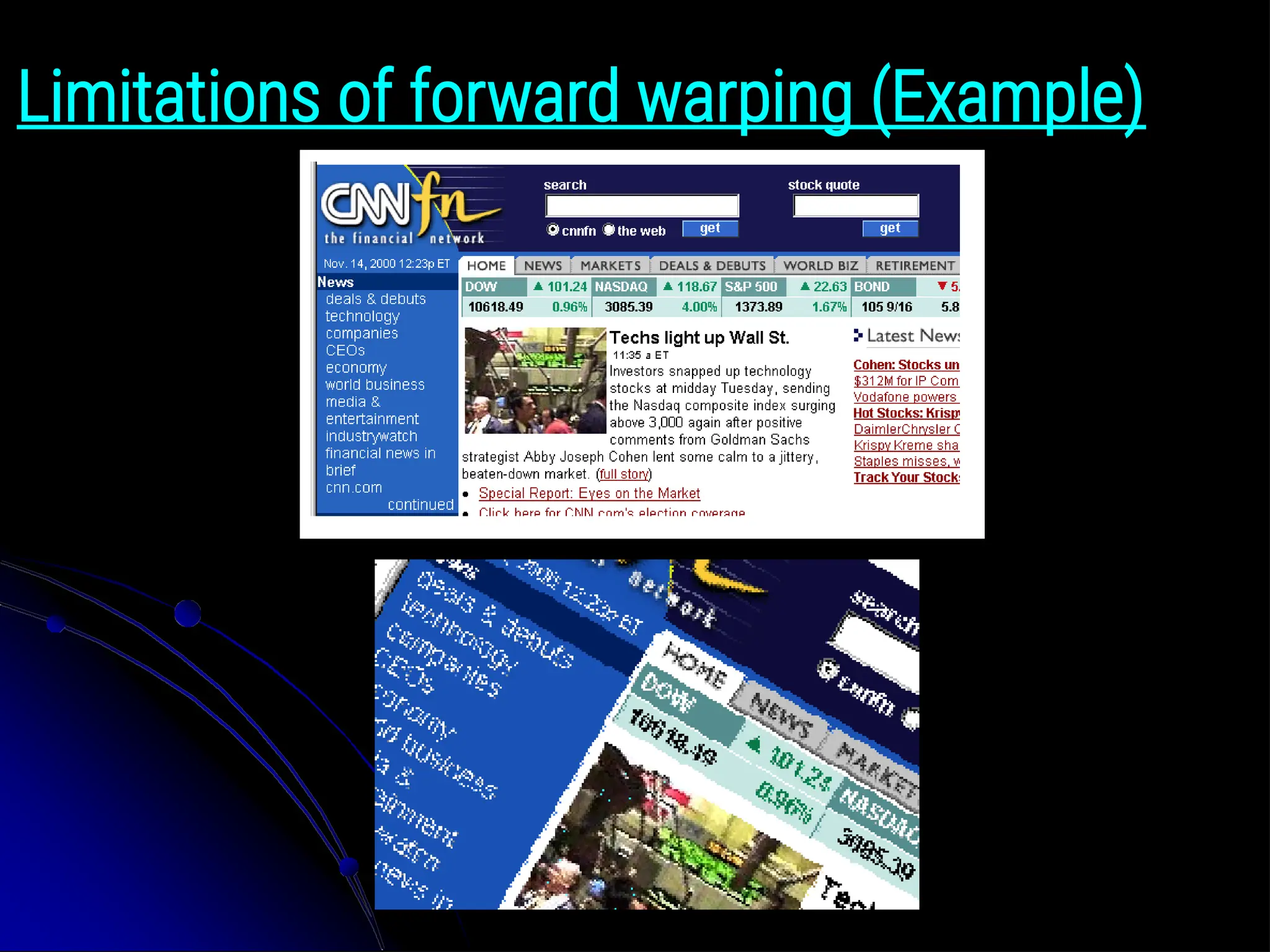
Limitations of forwardwarping ● Rounding the value of x` to the nearest integer coordinate and copy the pixel there, but the resulting image has severe aliasing and pixels that jump around a lot when animating the transformation. ● You can also “distribute” the value among its four nearest neighbors in a weighted (bilinear) fashion, keeping track of the per-pixel weights and normalizing at the end. ● This technique is called splatting and is sometimes used for volume rendering in the graphics community. ● The second major problem with forward warping is the appearance of cracks and holes, especially when magnifying an image. ● Filling such holes with their nearby neighbors can lead to further aliasing and blurring.
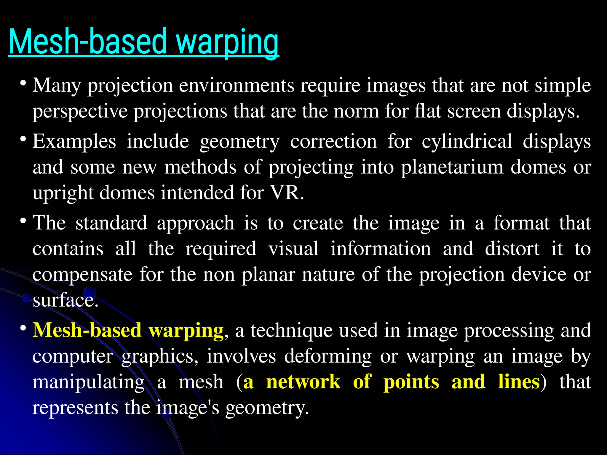
Mesh-based warping ● Many projectionenvironments require images that are not simple perspective projections that are the norm for flat screen displays. ● Examples include geometry correction for cylindrical displays and some new methods of projecting into planetarium domes or upright domes intended for VR. ● The standard approach is to create the image in a format that contains all the required visual information and distort it to compensate for the non planar nature of the projection device or surface. ● Mesh-based warping, a technique used in image processing and computer graphics, involves deforming or warping an image by manipulating a mesh (a network of points and lines) that represents the image's geometry.
106.
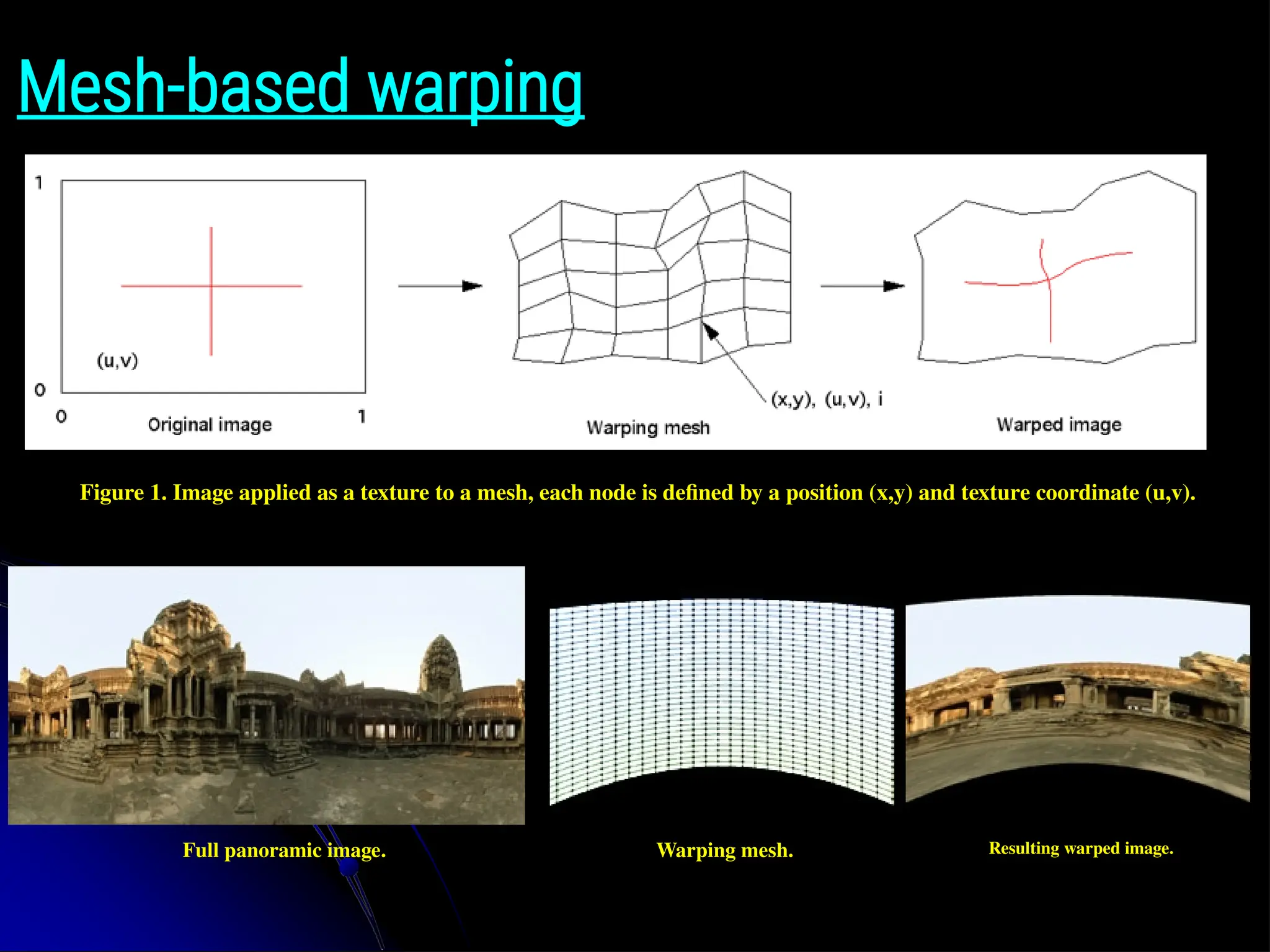
Mesh-based warping Figure 1.Image applied as a texture to a mesh, each node is defined by a position (x,y) and texture coordinate (u,v). Full panoramic image. Warping mesh. Resulting warped image.
107.
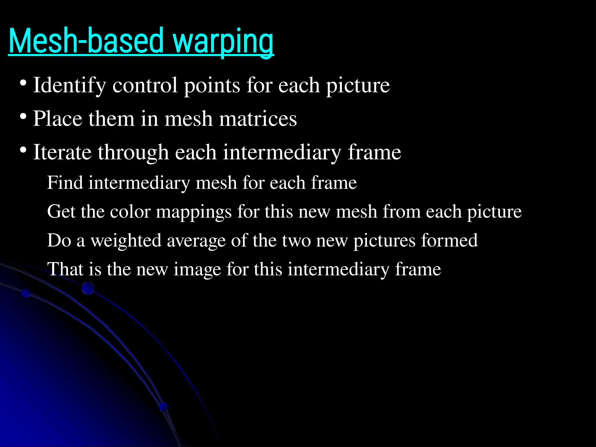
Mesh-based warping ● Identify controlpoints for each picture ● Place them in mesh matrices ● Iterate through each intermediary frame ● Find intermediary mesh for each frame ● Get the color mappings for this new mesh from each picture ● Do a weighted average of the two new pictures formed ● That is the new image for this intermediary frame
108.
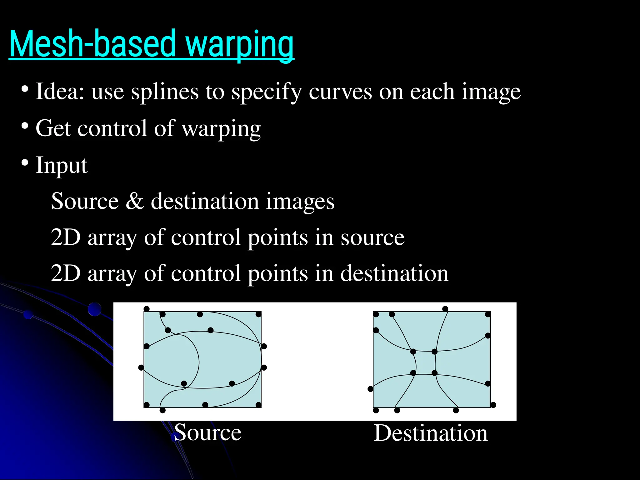
Mesh-based warping ● Idea: usesplines to specify curves on each image ● Get control of warping ● Input ● Source & destination images ● 2D array of control points in source ● 2D array of control points in destination Source Destination
109.
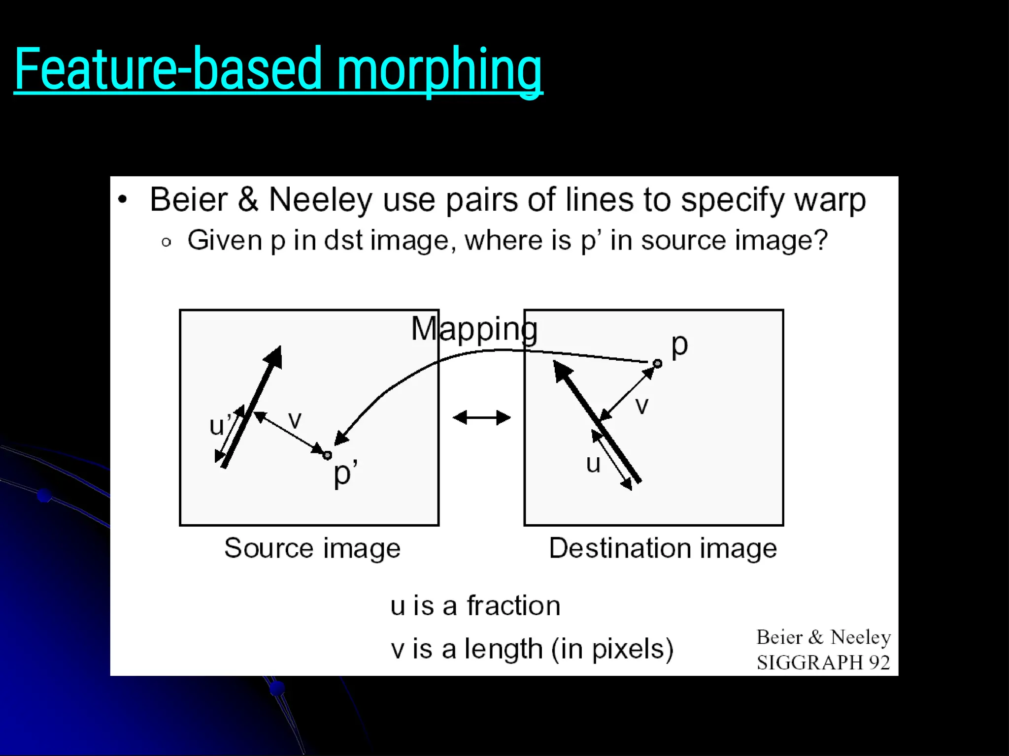
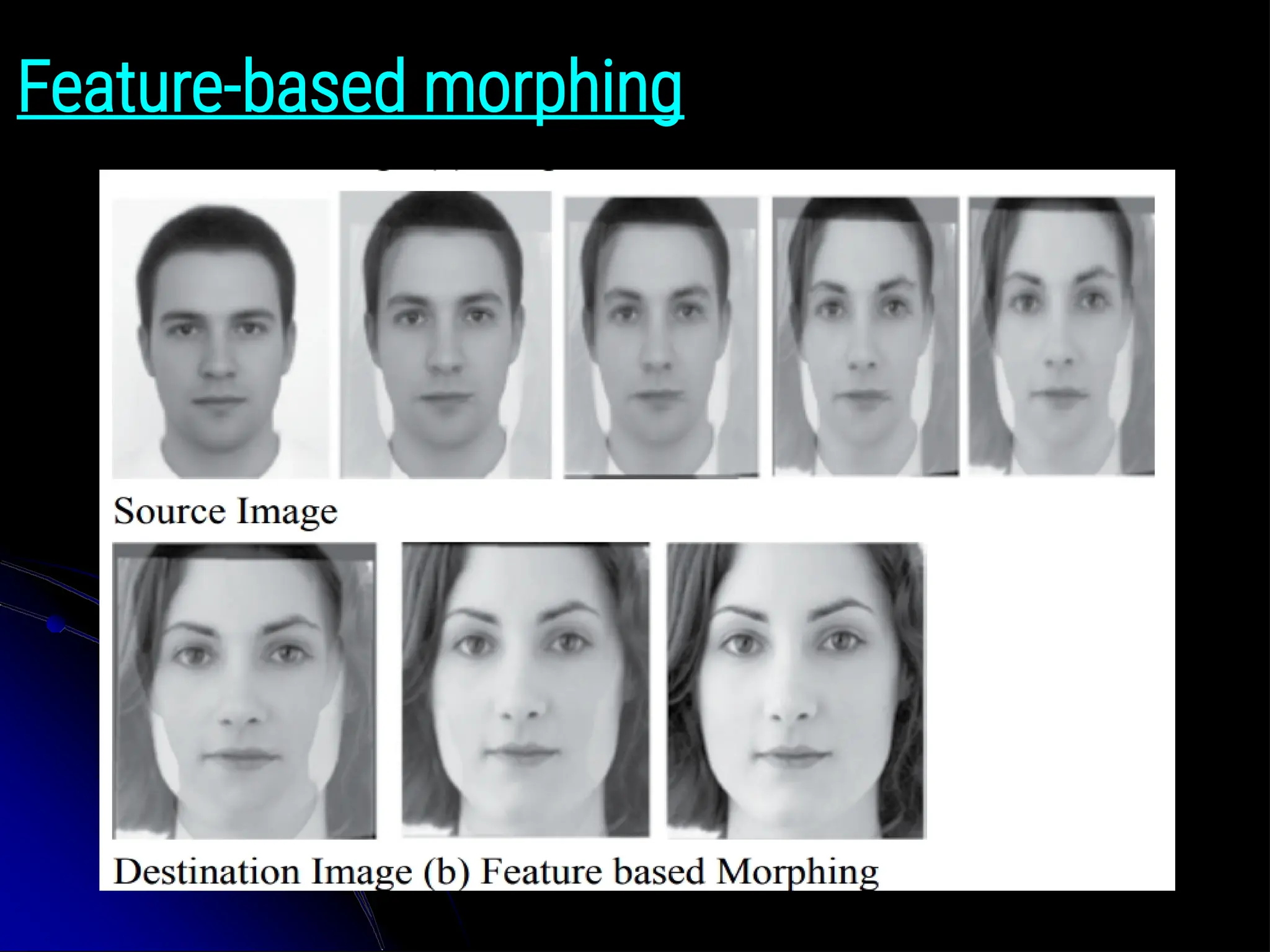
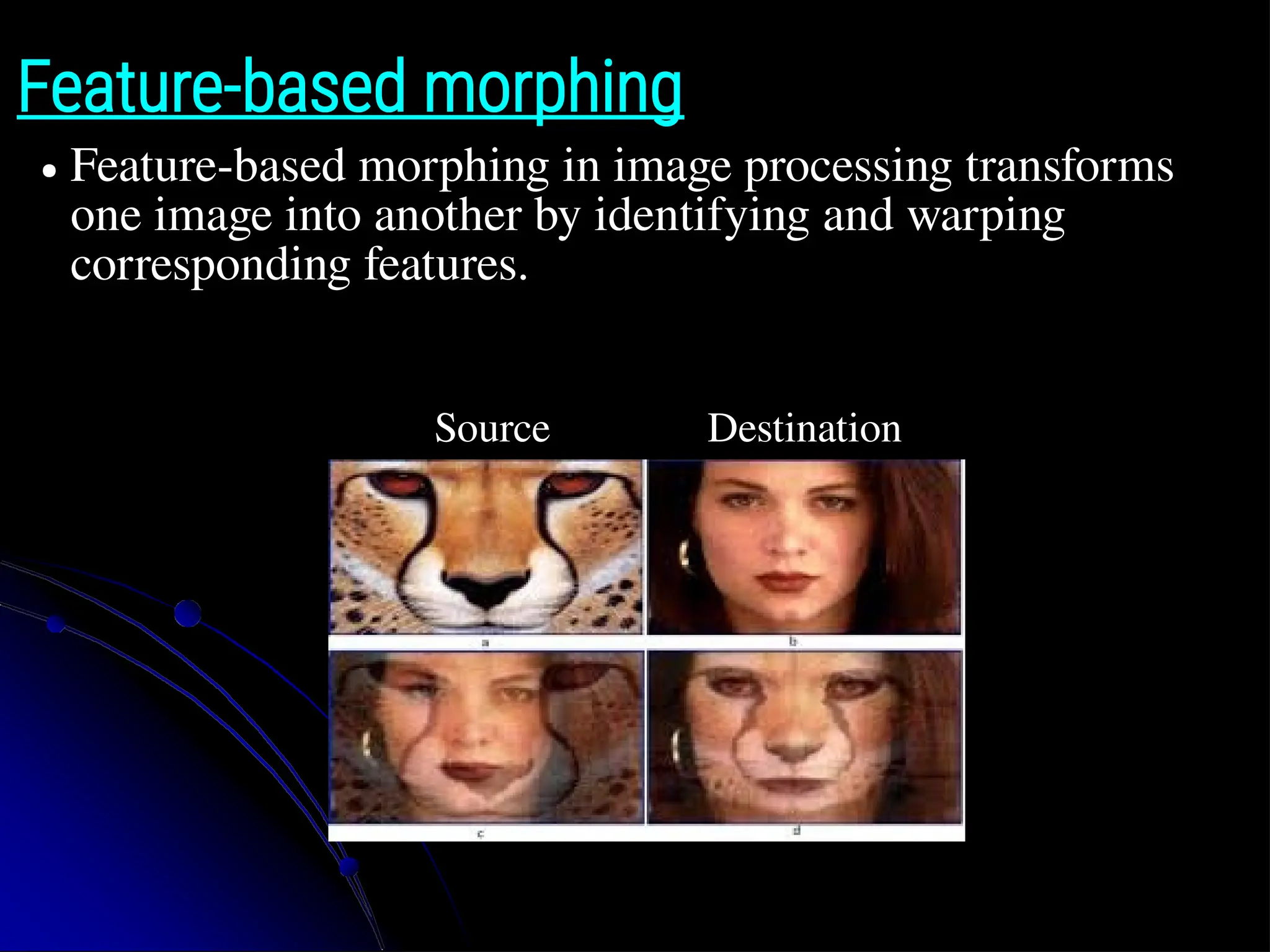
Feature-based morphing ● Feature-basedmorphing in image processing transforms one image into another by identifying and warping corresponding features. Source Destination
110.
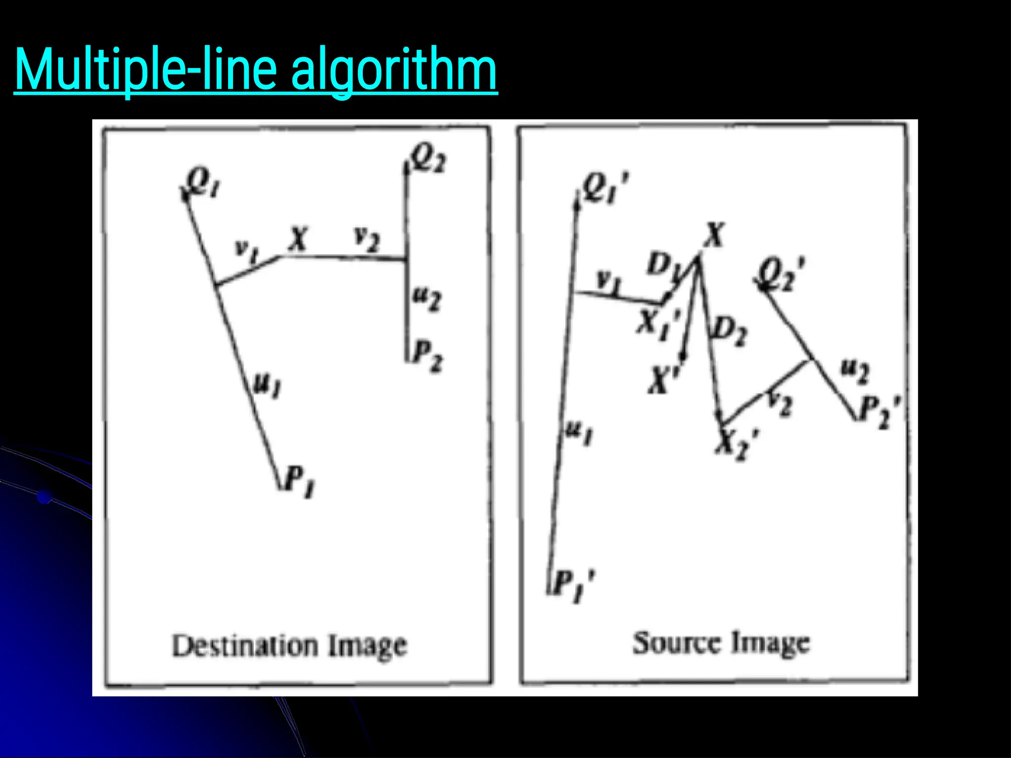
Feature-based morphing Step 1:Select lines in source image Is and Destination Image Id. Step 2: Generate intermediate frame I by generating new set of line segments by interpolating lines from their positions in Is to positions in Id. Step 3: Now intermediate frame I pixels in each line segments map to frame Is pixels by multiple line algorithm. Step 4: Multiple line algorithm: For each pixel X in the destination Find the corresponding weights in source Step 5: Now warped image Is and warped image Id is cross dissolved with given dissolution factor [0-1].

![Basics of Fourier transforms ● For a sinusoidal signal, ● where f is the frequency of signal, and if its frequency domain is taken, we can see a spike at f, and angular frequency ω = 2πf, and phase φi. ● If signal is sampled to form a discrete signal, we get the same frequency domain, but is periodic in the range [-π, π], or [0, 2π] or [0, N] in for N-point DFT). ● You can consider an image as a signal which is sampled in two directions. ● So taking Fourier transform in both X and Y directions gives you the frequency representation of image.](https://image.slidesharecdn.com/module-2computervisioncomplete-250417151638-8d7a6c49/75/Module-2-Computer-Vision-Image-Processing-40-2048.jpg)
![Feature-based morphing Step 1: Select lines in source image Is and Destination Image Id. Step 2: Generate intermediate frame I by generating new set of line segments by interpolating lines from their positions in Is to positions in Id. Step 3: Now intermediate frame I pixels in each line segments map to frame Is pixels by multiple line algorithm. Step 4: Multiple line algorithm: For each pixel X in the destination Find the corresponding weights in source Step 5: Now warped image Is and warped image Id is cross dissolved with given dissolution factor [0-1].](https://image.slidesharecdn.com/module-2computervisioncomplete-250417151638-8d7a6c49/75/Module-2-Computer-Vision-Image-Processing-110-2048.jpg)