2
$\begingroup$

I would like to plot the intersection between the surface $z=-\frac{y}{2}+1$ and the surface $z=\sqrt{1-x^{2}}$.

This is what I tried:

A1 := ParametricPlot3D[{Sqrt[1 - z^2], y, z}, {y, 0, 2}, {z, 0, -y/2 + 1}, PlotStyle -> {Red}, PlotStyle -> Thickness[0.02], AxesStyle -> Thick, Boxed -> False, AxesOrigin -> {0, 0, 0}, AxesLabel -> {x, y, z}]; A2 := ParametricPlot3D[{-Sqrt[1 - z^2], y, z}, {y, 0, 2}, {z, 0, -y/2 + 1}, PlotStyle -> {Red}, PlotStyle -> Thickness[0.02], AxesStyle -> Thick, Boxed -> False, AxesOrigin -> {0, 0, 0}, AxesLabel -> {x, y, z}]; A3 := ParametricPlot3D[{x, y, -y/2 + 1}, {y, 0, 2}, {x, -Sqrt[y - y^2/4], Sqrt[y - y^2/4]}, PlotStyle -> {Blue}, PlotStyle -> Thickness[0.02], AxesStyle -> Thick, Boxed -> False, AxesOrigin -> {0, 0, 0}, AxesLabel -> {x, y, z}]; Show[A1, A2, A3] 

Here is the picture:

enter image description here

My question: how can we remove the white gap shown in the picture?

Thanks for any hint.

$\endgroup$
4
  • 2
    $\begingroup$ Add PlotPoints->100 in A3-plot! $\endgroup$ Commented Jan 20, 2020 at 10:46
  • $\begingroup$ One would refine the plotting more by increasing the plot points by adding an option: PlotPoints -> 100 for example $\endgroup$ Commented Jan 20, 2020 at 10:46
  • $\begingroup$ @Ulrich That is so great. $\endgroup$ Commented Jan 20, 2020 at 10:50
  • $\begingroup$ The proper way is to get them to use exactly the same vertices on the edge. It's not a simple matter to get them to do it. Even with a lot of plot points, you still get the background showing through sometimes. And if you want to create a region with it, you need to close up the holes. $\endgroup$ Commented Jan 20, 2020 at 14:29

3 Answers 3

1
$\begingroup$

The OP's solution is doing too much work. In fact, this picture can be generated with a single Plot3D[] call, through the judicious use of Min[] and a straightforward ColorFunction construction:

Plot3D[Min[Sqrt[1 - x^2], 1 - y/2], {x, -1, 1}, {y, 0, 2}, ColorFunction -> Function[{x, y, z}, If[(1 - y/2)^2 < 1 - x^2, Blue, Red]], ColorFunctionScaling -> False, Exclusions -> None, PlotPoints -> 75] 

plot of cut-off surface

$\endgroup$
1
$\begingroup$

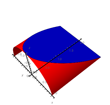
Here's a way, but you lose the misaligned mesh lines:

A1 = ParametricPlot3D[{Sqrt[1 - z^2], y, z}, {y, 0, 2}, {z, 0, -y/2 + 1}, PlotStyle -> {Red}, PlotStyle -> Thickness[0.02], AxesStyle -> Thick, Boxed -> False, AxesOrigin -> {0, 0, 0}, AxesLabel -> {x, y, z}, Mesh -> None, BoundaryStyle -> Green]; A2 = ParametricPlot3D[{-Sqrt[1 - z^2], y, z}, {y, 0, 2}, {z, 0, -y/2 + 1}, PlotStyle -> {Red}, PlotStyle -> Thickness[0.02], AxesStyle -> Thick, Boxed -> False, AxesOrigin -> {0, 0, 0}, AxesLabel -> {x, y, z}, Mesh -> None, BoundaryStyle -> Green]; boundaryPoints = Join[ First@Cases[Normal@A1, Line[p_] :> DeleteCases[p, {x_Real, y_Real, z_Real} /; (z == 0 && y != 2) || (y == 0 && z != 0 && z != 1)], Infinity], Reverse@First@Cases[Normal@A2, Line[p_] :> DeleteCases[p, {x_Real, y_Real, z_Real} /; (z == 0 && y != 2) || (y == 0 && z != 0 && z != 1)], Infinity] ]; Show[ DeleteCases[A1, _Line, Infinity], (* remove green boundary *) DeleteCases[A2, _Line, Infinity], Graphics3D[{Blue, Polygon@boundaryPoints}] ] 

enter image description here

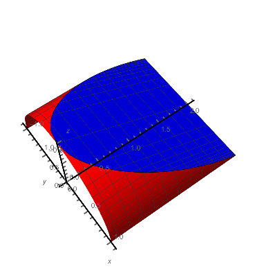
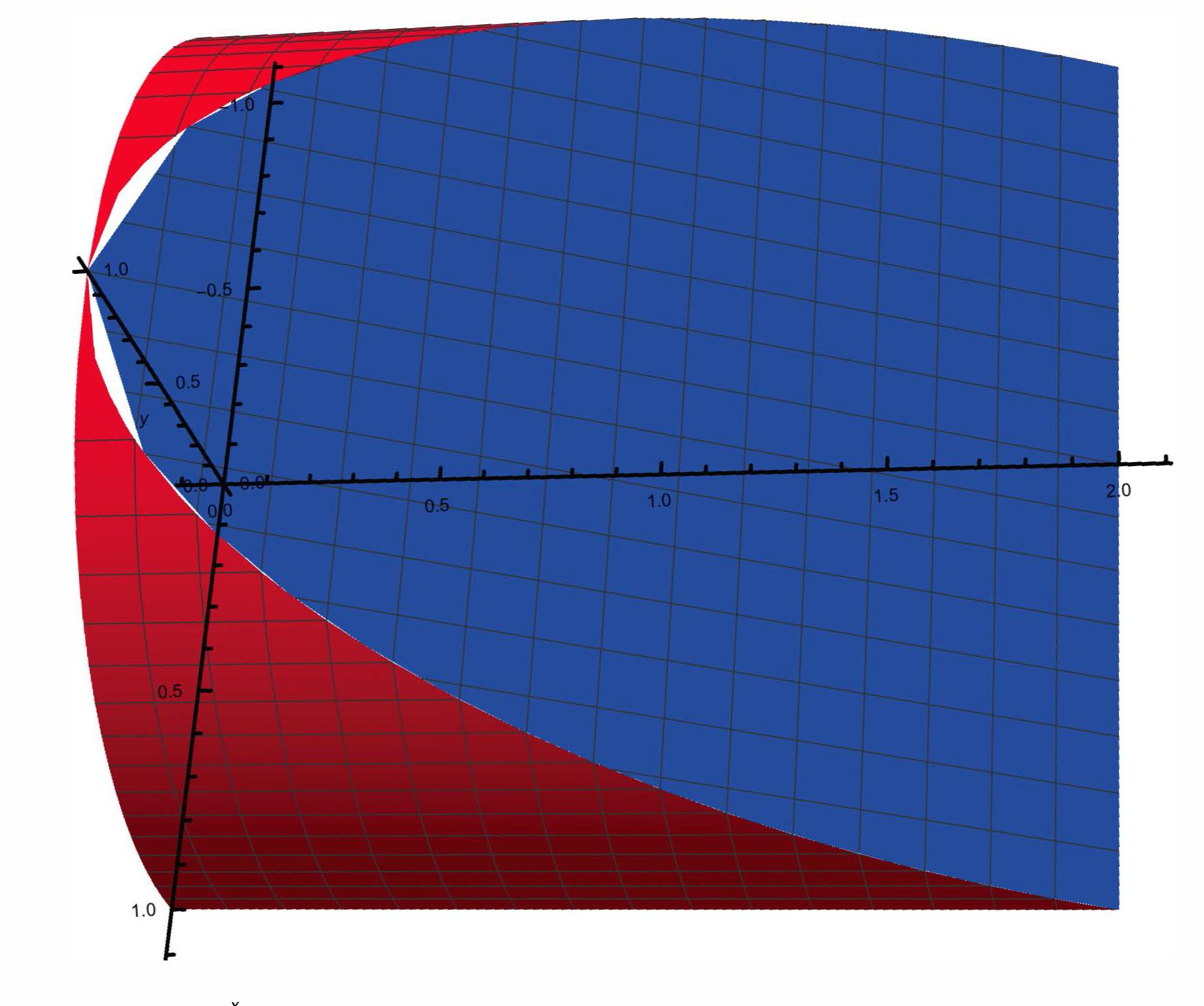
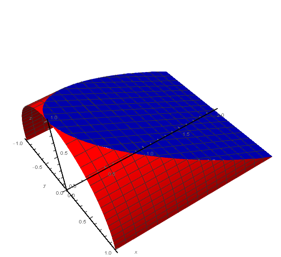
Here's a way to get the meshes aligned:

A1 = ParametricPlot3D[{Sqrt[1 - z^2], y, z}, {y, 0, 2}, {z, 0, -y/2 + 1}, PlotStyle -> {Red}, PlotStyle -> Thickness[0.02], AxesStyle -> Thick, Boxed -> False, AxesOrigin -> {0, 0, 0}, AxesLabel -> {x, y, z}, Mesh -> None, BoundaryStyle -> Green]; ypts = Cases[Normal@A1, Line[p_] :> DeleteCases[p, {x_Real, y_Real, z_Real} /; (z == 0 && y != 2) || (y == 0 && z != 0 && z != 1)], Infinity][[1, All, 2]] // DeleteDuplicates; mf = {#2 &, #3 &}; mesh = {Subdivide[-2, 2, 21], Subdivide[0, 1, 11]}; A3 = ListPlot3D[Flatten[Table[ Table[{x, y, -y/2 + 1}, {x, Subdivide[-Sqrt[y - y^2/4], Sqrt[y - y^2/4], Sqrt[y - y^2/4]/16 /. {dx_ /; dx == 0 :> 1, _ -> 10}]}], {y, ypts}], 1], PlotStyle -> {Blue}, PlotStyle -> Thickness[0.02], AxesStyle -> Thick, AxesOrigin -> {0, 0, 0}, AxesLabel -> {x, y, z}, MeshFunctions -> {#1 &, #2 &}, Mesh -> {Join[-#, #] &@Sqrt[1 - Last@mesh^2], First@mesh}]; A1 = ParametricPlot3D[{Sqrt[1 - z^2], y, z}, {y, 0, 2}, {z, 0, -y/2 + 1}, PlotStyle -> {Red}, PlotStyle -> Thickness[0.02], AxesStyle -> Thick, Boxed -> False, AxesOrigin -> {0, 0, 0}, AxesLabel -> {x, y, z}, MeshFunctions -> {#2 &, #3 &}, Mesh -> mesh]; Show[ A1, A1 /. (* reflect A1 and its VertexNormals *) GraphicsComplex[p_, g_, opts___] :> GraphicsComplex[p.DiagonalMatrix[{-1, 1, 1}], g, {opts} /. HoldPattern[VertexNormals -> v_] :> VertexNormals -> v.DiagonalMatrix[-{-1, 1, 1}]], A3] 
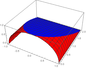
enter image description here

$\endgroup$
1
$\begingroup$
ClearAll[fa, fb, fc] fa[x_] := -x/2 + 1 fb[x_] := Sqrt[1 - x^2] fc[x_] := Sqrt[x - x^2/4]; 
  1. You can generate the two red surfaces using a single ParametricPlot3D.
  2. You can use the option RegionFunction instead of making the range of the second parameter depend on the value of the first parameter.

p1 = ParametricPlot3D[{{fb[y], x, y}, {- fb[y], x, y}}, {x, 0, 2}, {y, 0, 1}, PlotStyle -> Red, AxesLabel -> {x, y, z}, AxesStyle -> Thick, Boxed -> False, AxesOrigin -> {0, 0, 0}, RegionFunction -> (0 < #3 <= fa[#2] &)]; p2 = ParametricPlot3D[{y, x, fa[x]}, {x, 0, 2}, {y, -1, 1}, PlotStyle -> Blue, RegionFunction -> (-fc[#2] <= # <= fc[#2] &)]; Show[p1, p2, ImageSize -> Large] 

enter image description here

$\endgroup$

Start asking to get answers

Find the answer to your question by asking.

Ask question

Explore related questions

See similar questions with these tags.