15
\$\begingroup\$

Introduction to Numerical Mathematics

This is the "Hello, World!" of PDEs (Partial Differential Equations). The Laplace or Diffusion Equation appears often in Physics, for example Heat Equation, Deforming, Fluid Dynamics, etc... As real life is 3D but we want to say "Hello, World!" and not sing "99 bottles of beer,..." this task is given in 1D. You may interpret this as a rubber robe tied to a wall on both ends with some force applied to it.

On a \$[0,1]\$ domain, find a function \$u\$ for given source function \$f\$ and boundary values \$u_L\$ and \$u_R\$ such that:

  • \$-u'' = f\$
  • \$u(0) = u_L\$
  • \$u(1) = u_R\$

\$u''\$ denotes the second derivative of \$u\$

This can be solved purely theoretically but your task is it to solve it numerically on a discretized domain \$x\$ for \$N\$ points:

  • \$x = \{\frac i {N-1} : 0 \le i \le N-1\}\$ or 1-based: \$\{\frac {i-1} {N-1} : 0 \le i \le N-1\}\$
  • \$h = \frac 1 {N-1}\$ is the spacing

Input

  • \$f\$ as a function, expression or string
  • \$u_L\$, \$u_R\$ as floating point values
  • \$N \ge 2\$ as an integer

Output

  • Array, List, some sort of separated string of \$u\$ such that \$u_i = u(x_i)\$

Examples

Example 1

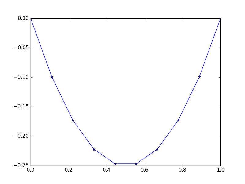
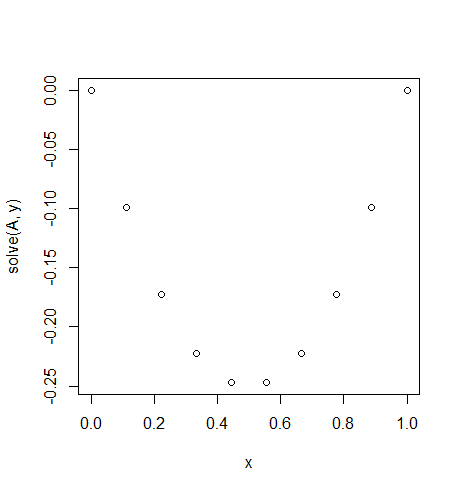
Input: \$f = -2\$, \$u_L = u_R = 0\$, \$N = 10\$ (Don't take \$f=-2\$ wrong, it is not a value but a constant function that returns \$-2\$ for all \$x\$. It is like a constant gravity force on our rope.)

Output: [-0.0, -0.09876543209876543, -0.1728395061728395, -0.22222222222222224, -0.24691358024691357, -0.24691358024691357, -0.22222222222222224, -0.1728395061728395, -0.09876543209876547, -0.0]

There exists an easy exact solution: \$u = -x(1-x)\$

Example 2

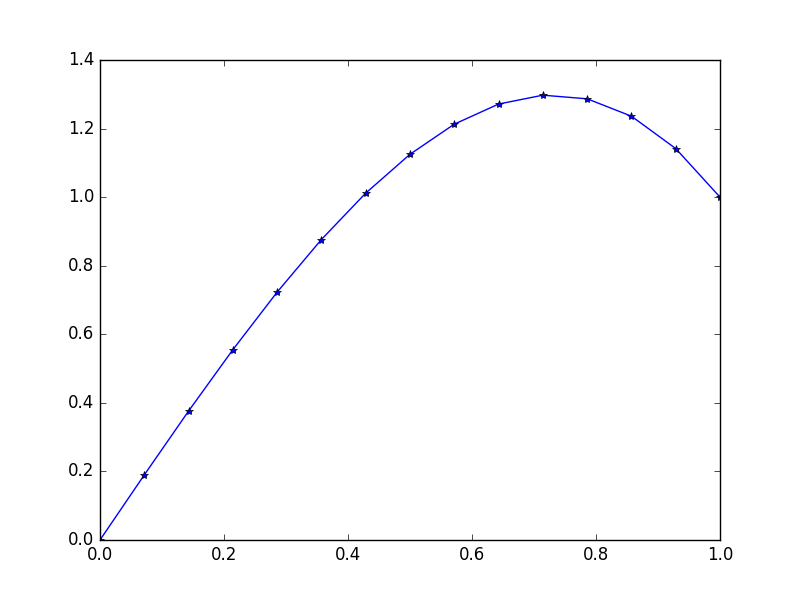
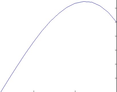
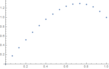
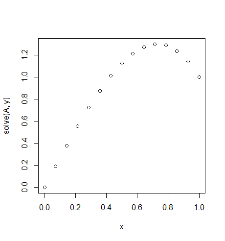
Input: \$f = 10x\$, \$u_L = 0\$, \$u_R = 1\$, \$N = 15\$ (Here there is a lot of upwind on the right side)

Output: [ 0., 0.1898688, 0.37609329, 0.55502915, 0.72303207, 0.87645773, 1.01166181, 1.125, 1.21282799, 1.27150146, 1.29737609, 1.28680758, 1.2361516, 1.14176385, 1.]

The exact solution for this states: \$u = \frac 1 3(8x-5x^3)\$

Example 3

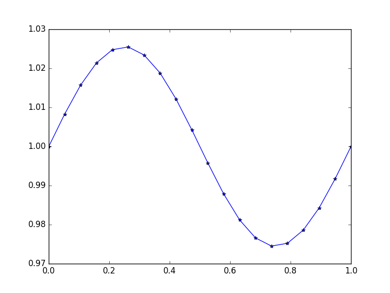
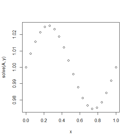
Input: \$f = \sin(2\pi x)\$, \$u_L = u_R = 1\$, \$N = 20\$ (Someone broke gravity or there is a sort of up- and downwind)

Output: [ 1., 1.0083001, 1.01570075, 1.02139999, 1.0247802, 1.0254751, 1.02340937, 1.01880687, 1.01216636, 1.00420743, 0.99579257, 0.98783364, 0.98119313, 0.97659063, 0.9745249, 0.9752198, 0.97860001, 0.98429925, 0.9916999, 1.]

Here the exact solution is \$u = \frac {\sin(2πx)} {4π^2}+1\$

Example 4

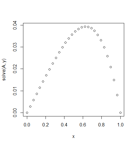
Input: \$f = \exp(x^2)\$, \$u_L = u_R = 0\$, \$N=30\$

Output: [ 0. 0.02021032 0.03923016 0.05705528 0.07367854 0.0890899 0.10327633 0.11622169 0.12790665 0.13830853 0.14740113 0.15515453 0.16153488 0.1665041 0.17001962 0.172034 0.17249459 0.17134303 0.16851482 0.1639387 0.15753606 0.1492202 0.13889553 0.12645668 0.11178744 0.09475961 0.07523169 0.05304738 0.02803389 0. ]

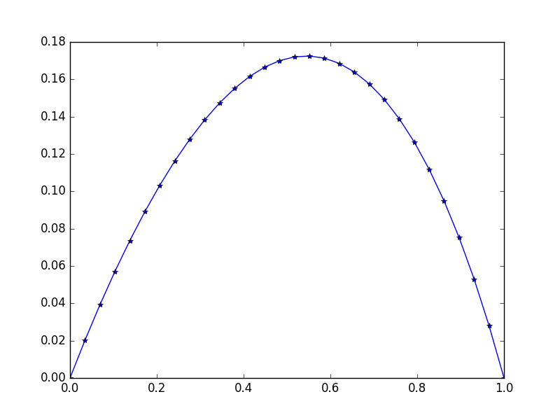
Note the slight asymmetry

FDM

One possible method to solve this is the Finite Difference Method:

  • Rewrite \$-u_i'' = f_i\$ as \$\frac {-u_{i-1} + 2u_i - u_{i+1}} {h^2} = f_i\$, which equals \$-u_{i-1} + 2u_i - u_{i+1} = h^2 f_i\$
  • Setup the equations:

$$ u_0 = u_L \\ \frac {-u_0 + 2u_1 - u_2} {h^2} = f_1 \\ \frac {-u_1 + 2u_2 - u_3} {h^2} = f_2 \\ \dots = \dots \\ \frac {-u_{n-3} + 2u_{n-2} - u_{n-1}} {h^2} = f_{n-2} \\ u_{n-1} = u_R $$

  • Which are equal to a matrix-vector equation:

$$ \begin{pmatrix} 1 & & & & & & \\ -1 & 2 & -1 & & & & \\ & -1 & 2& -1& & & \\ & & \ddots & \ddots & \ddots & & \\ & & & -1 & 2 & -1 & \\ & & & & -1 & 2 & -1 \\ & & & & & & 1 \end{pmatrix} \begin{pmatrix} u_0 \\ u_1 \\ u_2 \\ \vdots \\ u_{n-3} \\ u_{n-2} \\ u_{n-1} \end{pmatrix} = \begin{pmatrix} u_L \\ h^2 f_1 \\ h^2 f_2 \\ \vdots \\ h^2 f_{n-3} \\ h^2 f_{n-2} \\ u_R \end{pmatrix} $$

  • Solve this equation and output the \$u_i\$

One implementation of this for demonstration in Python:

import matplotlib.pyplot as plt import numpy as np def laplace(f, uL, uR, N): h = 1./(N-1) x = [i*h for i in range(N)] A = np.zeros((N,N)) b = np.zeros((N,)) A[0,0] = 1 b[0] = uL for i in range(1,N-1): A[i,i-1] = -1 A[i,i] = 2 A[i,i+1] = -1 b[i] = h**2*f(x[i]) A[N-1,N-1] = 1 b[N-1] = uR u = np.linalg.solve(A,b) plt.plot(x,u,'*-') plt.show() return u print laplace(lambda x:-2, 0, 0, 10) print laplace(lambda x:10*x, 0, 1, 15) print laplace(lambda x:np.sin(2*np.pi*x), 1, 1, 20) 

Alternative implementation without Matrix Algebra (using the Jacobi method)

def laplace(f, uL, uR, N): h=1./(N-1) b=[f(i*h)*h*h for i in range(N)] b[0],b[-1]=uL,uR u = [0]*N def residual(): return np.sqrt(sum(r*r for r in[b[i] + u[i-1] - 2*u[i] + u[i+1] for i in range(1,N-1)])) def jacobi(): return [uL] + [0.5*(b[i] + u[i-1] + u[i+1]) for i in range(1,N-1)] + [uR] while residual() > 1e-6: u = jacobi() return u 

You may however use any other method to solve the Laplace equation. If you use an iterative method, you should iterate until the residual \$|b-Au| < 10^{-6}\$, with \$b\$ being the right hand side vector \$u_L,f_1 h^2,f_2 h^2, \dots\$

Notes

Depending on your solution method you may not solve the examples exactly to the given solutions. At least for \$N \to \infty\$ the error should approach zero.

Standard loopholes are disallowed, built-ins for PDEs are allowed.

Bonus

A bonus of -30% for displaying the solution, either graphical or ASCII-art.

Winning

This is codegolf, so shortest code in bytes wins!

\$\endgroup\$
6
  • \$\begingroup\$ I recommend adding an example which is not analytically solvable, e.g. with f(x) = exp(x^2). \$\endgroup\$ Commented Nov 7, 2016 at 9:27
  • \$\begingroup\$ @flawr Sure, it has a solution however the error function is involved. \$\endgroup\$ Commented Nov 7, 2016 at 9:41
  • 1
    \$\begingroup\$ Sorry, that was perhaps the wrong expression, might "non-elementary antiderivative" be better suited? I mean functions like log(log(x)) or sqrt(1-x^4) which do have an integral, which is however not expressible in elementary functions. \$\endgroup\$ Commented Nov 7, 2016 at 9:46
  • \$\begingroup\$ @flawr No it is fine, the error function is not elementary, I just wanted to say there is a way to express the solution analytically but u(x) = 1/2 (-sqrt(π) x erfi(x)+sqrt(π) erfi(1) x+e^(x^2)-e x+x-1) is not exactly calculable. \$\endgroup\$ Commented Nov 7, 2016 at 9:48
  • \$\begingroup\$ Why iterate until 1e-6 and not iterate until 1e-30? \$\endgroup\$ Commented Nov 8, 2016 at 10:43

5 Answers 5

6
\$\begingroup\$

Matlab, 84, 81.2 79.1 bytes = 113 - 30%

function u=l(f,N,a,b);A=toeplitz([2,-1,(3:N)*0]);A([1,2,end-[1,0]])=eye(2);u=[a,f((1:N-2)/N)*(N-1)^2,b]/A;plot(u) 

Note that in this example the I use row vectors, this means that the matrix A is transposed. f is taken as a function handle, a,b are the left/right side Dirichlet contraints.

function u=l(f,N,a,b); A=toeplitz([2,-1,(3:N)*0]); % use the "toeplitz" builtin to generate the matrix A([1,2,end-[1,0]])=eye(2); % adjust first and last column of matrix u=[a,f((1:N-2)/N)*(N-1)^2,b]/A; % build right hand side (as row vector) and right mu plot(u) % plot the solution 

For the example f = 10*x, u_L = 0 u_R = 1, N = 15 this results in:

\$\endgroup\$
4
\$\begingroup\$

Mathematica, 52.5 bytes (= 75 * (1 - 30%))

+0.7 bytes per @flawr 's comment.

ListPlot[{#,u@#}&/@Subdivide@#4/.NDSolve[-u''@x==#&&u@0==#2&&u@1==#3,u,x]]& 

This plots the output.

e.g.

ListPlot[ ... ]&[10 x, 0, 1, 15] 

enter image description here

Explanation

NDSolve[-u''@x==#&&u@0==#2&&u@1==#3,u,x] 

Solve for the function u.

Subdivide@#4 

Subdivide the interval [0,1] into N (4th input) parts.

{#,u@#}&/@ ... 

Map u to the output of Subdivide.

ListPlot[ ... ] 

Plot the final result.

Non-graphing solution: 58 bytes

u/@Subdivide@#4/.NDSolve[-u''@x==#&&u@0==#2&&u@1==#3,u,x]& 
\$\endgroup\$
2
  • \$\begingroup\$ This does not work for f(x) = exp(x^2) \$\endgroup\$ Commented Nov 7, 2016 at 9:24
  • \$\begingroup\$ Perhaps you might want to use NDSolve for the general case of non elementary solutions. \$\endgroup\$ Commented Nov 7, 2016 at 10:54
3
\$\begingroup\$

R, 123.2 102.9 98.7 bytes (141-30%)

Edit: Saved a handful of bytes thanks to @Angs!

If someone wants to edit the pictures feel free to do so. This is basically an R adaptation of both the matlab and python versions posted.

function(f,a,b,N){n=N-1;x=1:N/n;A=toeplitz(c(2,-1,rep(0,N-2)));A[1,1:2]=1:0;A[N,n:N]=0:1;y=n^-2*sapply(x,f);y[1]=a;y[N]=b;plot(x,solve(A,y))} 

Ungolfed & explained:

u=function(f,a,b,N){ n=N-1; # Alias for N-1 x=0:n/n; # Generate the x-axis A=toeplitz(c(2,-1,rep(0,N-2))); # Generate the A-matrix A[1,1:2]=1:0; # Replace first row-- A[N,n:N]=0:1; # Replace last row y=n^-2*sapply(x,f) # Generate h^2*f(x) y[1]=a;y[N]=b; # Replace first and last elements with uL(a) and uR(b) plot(x,solve(A,y)) # Solve the matrix system A*x=y for x and plot against x } 

Example & test cases:

The named and ungolfed function can be called using:

u(function(x)-2,0,0,10) u(function(x)x*10,0,1,15) u(function(x)sin(2*pi*x),1,1,20) u(function(x)x^2,0,0,30) 

Note that the f argument is an R-function.

To run the golfed version simply use (function(...){...})(args)

enter image description here enter image description here enter image description here enter image description here

\$\endgroup\$
7
  • \$\begingroup\$ I think you can drop the is.numeric(f) check if you declare f as function, it is no requirement to pass it directly in the function call to the solver. \$\endgroup\$ Commented Nov 7, 2016 at 15:57
  • \$\begingroup\$ Ah I see, I did not know there is a difference between those two. Well, if it shorter you can modify your solver to accept f as a function so you don't have to check for the case it is a constant (function). \$\endgroup\$ Commented Nov 7, 2016 at 16:25
  • 1
    \$\begingroup\$ @Billywob there's no need for f to ever be numeric. f = (function(x)-2) works for the first example, so there's never a need to rep. \$\endgroup\$ Commented Nov 7, 2016 at 16:52
  • \$\begingroup\$ You can use x<-0:10/10;f<-function(x){-2};10^-2*sapply(x,f) if f(x) isn't quaranteed to be vectorized or just 10^-2*f(x) if f is vectorized (laplace(Vectorize(function(x)2),0,0,10) \$\endgroup\$ Commented Nov 7, 2016 at 17:07
  • \$\begingroup\$ Don't use eval, give f as a proper function. \$\endgroup\$ Commented Nov 7, 2016 at 17:08
2
\$\begingroup\$

Haskell, 195 168 bytes

import Numeric.LinearAlgebra p f s e n|m<-[0..]!!n=((n><n)(([1,0]:([3..n]>>[[-1,2,-1]])++[[0,1]])>>=(++(0<$[3..n]))))<\>(col$s:map((/(m-1)^2).f.(/(m-1)))[1..m-2]++[e]) 

The readability took quite a hit. Ungolfed:

laplace f start end _N = linearSolveLS _M y where n = fromIntegral _N _M = (_N><_N) --construct n×n matrix from list ( ( [1,0] --make a list of [1,0] : ([3.._N]>>[[-1,2,-1]]) -- (n-2)×[-1,2,-1] ++ [[0,1]]) -- [0,1] >>= (++(0<$[3.._N])) --append (n-2) zeroes and concat ) --(m><n) discards the extra zeroes at the end h = 1/(n-1) :: Double y = asColumn . fromList $ start : map ((*h^2).f.(*h)) [1..n-2] ++ [end] 

TODO: Printing in 83 71 bytes.

Lemme see:

import Graphics.Rendering.Chart.Easy import Graphics.Rendering.Chart.Backend.Cairo 

D'oh!

\$\endgroup\$
3
  • \$\begingroup\$ I dont know much about Haskell, but perhaps the solution without matrix algebra might be shorter, I added a second sample implementation. \$\endgroup\$ Commented Nov 7, 2016 at 17:45
  • \$\begingroup\$ @KarlNapf doesn't come very close This is only semi-golfed but it has to use a lot of verbose built-in functions. With matrix algebra most of the code is building the matrix (64 bytes) and the import (29 bytes). The residual and jacobi take quite a lot space. \$\endgroup\$ Commented Nov 7, 2016 at 19:04
  • \$\begingroup\$ Well, too bad but it was worth a try. \$\endgroup\$ Commented Nov 7, 2016 at 19:09
1
\$\begingroup\$

Axiom, 579 460 bytes

l(w,y)==(r:=0;for i in 1..y|index?(i,w)repeat r:=i;r) g(z:EQ EXPR INT,y:BasicOperator,a0:Float,a1:Float,a2:Float):Float==(r:=digits();digits(r+30);q:=seriesSolve(z,y,x=0,[a,b])::UTS(EXPR INT,x,0);w:=eval(q,0);s:=l(w,r+30);o:=solve([w.s=a0,eval(q,1).s=a1]::List(EQ POLY Float),[a,b]);v:=eval(eval(eval(q,a2).s,o.1.1),o.1.2);digits(r);v) m(z:EXPR INT,a0:Float,a1:Float,n:INT):List Float==(n:=n-1;y:=operator 'y;r:=[g(D(y x,x,2)=-z,y,a0,a1,i/n)for i in 0..n];r) 

ungolf it and test

Len(w,y)==(r:=0;for i in 1..y|index?(i,w)repeat r:=i;r) -- g(z,a0,a1,a2) -- Numeric solve z as f(y''(x),y'(x),y(x))=g(x) with ini conditions y(0)=a0 y(1)=a1 in x=a2 NSolve2order(z:EQ EXPR INT,y:BasicOperator,a0:Float,a1:Float,a2:Float):Float== r:=digits();digits(r+30) q:=seriesSolve(z,y,x=0,[a,b])::UTS(EXPR INT,x,0) w:=eval(q,0);s:=Len(w,r+30) o:=solve([w.s=a0,eval(q,1).s=a1]::List(EQ POLY Float),[a,b]) v:=eval(eval(eval(q,a2).s,o.1.1),o.1.2);digits(r) v InNpoints(z:EXPR INT,a0:Float,a1:Float,n:INT):List Float==(n:=n-1;y:=operator 'y;r:=[NSolve2order(D(y x,x,2)=-z,y,a0,a1,i/n)for i in 0..n];r) 

the function for the question is m(,,,) the above code is put in the file "file.input" and load in Axiom. The result depends from the digits() function.

if some one think it is not golfed => he or she can show how to do it... thanks

PS

it seems the 6 numbers afther the . for e^(x^2) are not ok here or in the examples but here i increase the digits but numbers not change... for me it means that numbers in example are wrong. Why all other has not showed their numbers?

for sin(2*%pi*x) there are problems too

"Here the exact solution is u = (sin(2*π*x))/(4*π^2)+1" i copyed the exact solution for x=1/19:

 (sin(2*π/19))/(4*π^2)+1 

in WolframAlpha https://www.wolframalpha.com/input/?i=(sin(2%CF%80%2F19))%2F(4%CF%80%5E2)%2B1 it result

1.008224733636964333380661957738992274267070440829381577926... 1.0083001 1234 1.00822473 

1.0083001 proposed as result is different in the 4th digit from the real result 1.00822473... (and not 6th)

-- in interactive mode (?) -> )read file (10) -> digits(9) (10) 10 Type: PositiveInteger (11) -> m(-2,0,0,10) (11) [0.0, - 0.0987654321, - 0.172839506, - 0.222222222, - 0.24691358, - 0.24691358, - 0.222222222, - 0.172839506, - 0.098765432, 0.0] Type: List Float (12) -> m(10*x,0,1,15) (12) [0.0, 0.189868805, 0.376093294, 0.555029155, 0.72303207, 0.876457726, 1.01166181, 1.125, 1.21282799, 1.27150146, 1.29737609, 1.28680758, 1.2361516, 1.14176385, 1.0] Type: List Float (13) -> m(sin(2*%pi*x),1,1,20) (13) [1.0, 1.00822473, 1.01555819, 1.02120567, 1.0245552, 1.02524378, 1.02319681, 1.0186361, 1.01205589, 1.00416923, 0.99583077, 0.987944112, 0.981363896, 0.976803191, 0.97475622, 0.975444804, 0.978794326, 0.98444181, 0.991775266, 1.0] Type: List Float (14) -> m(exp(x^2),0,0,30) (14) [0.0, 0.0202160702, 0.0392414284, 0.0570718181, 0.0737001105, 0.0891162547, 0.103307204, 0.116256821, 0.127945761, 0.138351328, 0.147447305, 0.155203757, 0.161586801, 0.166558343, 0.170075777, 0.172091643, 0.172553238, 0.171402177, 0.168573899, 0.163997099, 0.157593103, 0.149275146, 0.13894757, 0.126504908, 0.111830857, 0.0947971117, 0.0752620441, 0.0530692118, 0.0280456602, - 0.293873588 E -38] Type: List Float 
\$\endgroup\$
2
  • \$\begingroup\$ The numerical solution differs from the exact solution because the FDM here is only second order, that means only polynomials up to order 2 can be represented exactly. So only the f=-2 example has a matching analytical and numerical solution. \$\endgroup\$ Commented Nov 13, 2016 at 11:01
  • \$\begingroup\$ here the numeric solution seems ok if i change digits to 80 or 70 -> g(sin(2*%pi*x),1,1,1/19) 1.0082247336 3696433338 0661957738 9922742670 7044082938 1577926908 950765832 the other number 1.0082247336 3696433338 0661957738 9922742670 7044082938 1577926... \$\endgroup\$ Commented Nov 13, 2016 at 21:52

Start asking to get answers

Find the answer to your question by asking.

Ask question

Explore related questions

See similar questions with these tags.