Mathematica wouldn't be much helpful if one applied only formulae calculated by hand.
Here we demonstrate how to calculate the desired geometric objects with the system having a definition of the curve r[t] :
r[t_] := {t, t^2, t^3}
now we call uT the unit tangent vector to r[t]. Since we'd like it only for real parameters we add an assumption to Simplify that t is a real number. Similarly we can do it for the normal vector vN[t] and the binormal vB[t] :
uT[t_] = Simplify[ r'[t] / Norm[ r'[t] ], t ∈ Reals]; vN[t_] = Simplify[ uT'[t]/ Norm[ uT'[t]], t ∈ Reals]; vB[t_] = Simplify[ Cross[r'[t], r''[t]] / Norm[ Cross[r'[t], r''[t]] ], t ∈ Reals];
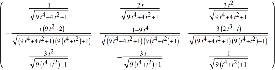
let's write down the formulae :
{uT[t], vN[t], vB[t]} // Column // TraditionalForm
Edit
Definitions provided above are clearly more useful than only to write them down. They are powerful enough to animate a moving reper along a curve r[t]. Indeed the vectors uT[t], vN[t] and vB[t] are orthogonal and normalized, e.g.
Simplify[ Norm /@ {uT[t], vN[t], vB[t]}, t ∈ Reals]
{1, 1, 1}
To demonstrate a moving reper we can use ParametricPlot3D and Arrow enclosed in Animate :
Animate[ Show[ ParametricPlot3D[ {r[t]}, {t, -1.3, 1.3}, PlotStyle -> {Blue, Thick}], Graphics3D[{ {Thick, Darker @ Red, Arrow[{r[s], r[s] + uT[s]}]}, {Thick, Darker @ Green, Arrow[{r[s], r[s] + vB[s]}]}, {Thick, Darker @ Cyan, Arrow[{r[s], r[s] + vN[s]}]}}], PlotRange -> {{-2, 2}, {-2, 2}, {-2, 2}}, ViewPoint -> {4, 6, 0}, ImageSize -> 600], {s, -1, 1}]