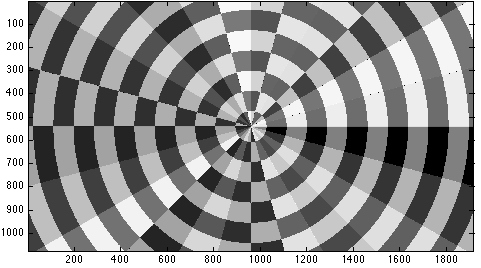
How can I generate such an image and fill every annular sector with a random colour?
How can I generate such an image and fill every annular sector with a random colour?
With V10 came RandomColor and ColorSpace
Using Michael E2's wonderful solution
plot = ParametricPlot[r {Cos[t], Sin[t]}, {r, 0, 12}, {t, 0, 2 Pi}, ImageSize -> 500, Mesh -> 13, MeshShading -> {{Red, Red}, {Red, Red}}, PlotRange -> {{-9, 9}, {-4, 4}}]; Grid @ Partition[Table[plot /. poly_Polygon :> {RandomColor[ColorSpace -> space], poly}, {space, {"RGB", "XYZ", "CMYK", "Grayscale"}}], 2] 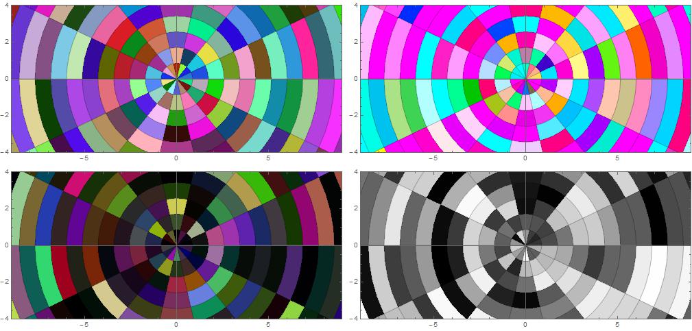
RandomColor and ColorSpace :) $\endgroup$ Hmm...Szabolcs beat me to it (in a comment) by one minute...
plot = ParametricPlot[r {Cos[t], Sin[t]}, {r, 0, 12}, {t, 0, 2 Pi}, Mesh -> 23, Axes -> False, MeshShading -> {{Red, Green}, {Blue, Yellow}}, PlotRange -> {{-9, 9}, {-4, 4}}]; plot /. poly_Polygon :> {RGBColor @@ RandomReal[1, 3], poly} 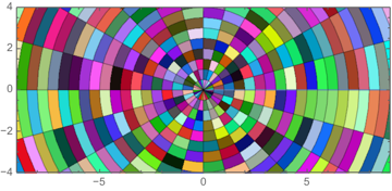
Making the MeshShading setting Dynamic also works without the need for post-processing:
ParametricPlot[r {Cos[t], Sin[t]}, {r, 0, 12}, {t, 0, 2 Pi}, Mesh -> 23, Axes -> False, MeshShading -> Dynamic@{{Hue@RandomReal[], Hue@RandomReal[]}, {Hue@RandomReal[], Hue@RandomReal[]}}, PlotRange -> {{-9, 9}, {-4, 4}}] 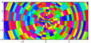
The same trick works in combination with V10 RandomColor:
ParametricPlot[r {Cos[t], Sin[t]}, {r, 0, 12}, {t, 0, 2 Pi}, Mesh -> 23, Axes -> False,BaseStyle->Opacity[.75], MeshShading ->Dynamic@ {{RandomColor[], RandomColor[]}, {RandomColor[], RandomColor[]}}, PlotRange -> {{-9, 9}, {-4, 4}}] 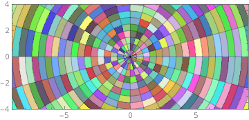
ParametricPlot[r {Cos[t], Sin[t]}, {r, 0, 12}, {t, 0, 2 Pi}, Mesh ->{25,25}, Axes -> False, BaseStyle->Opacity[.75], MeshShading ->Dynamic@Evaluate@ Table[RandomColor[],{25},{2}], PlotRange -> {{-9, 9}, {-4, 4}}] 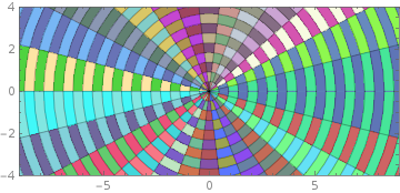
ParametricPlot[r {Cos[t], Sin[t]}, {r, 0, 12}, {t, 0, 2 Pi}, Mesh ->{25,25}, Axes -> False, BaseStyle->Opacity[.75], MeshShading ->Dynamic@Evaluate@ Table[RandomColor[],{2},{25}], PlotRange -> {{-9, 9}, {-4, 4}}] 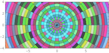
Dynamic), innovative and upvoteable :) $\endgroup$ FrontEnd -- as the owner/manager of Dynamic stuff -- triggers new calls to RandomReal/RandomColor since a given call changes something visible ..? Thanks for the vote by the way. $\endgroup$ InputForm of the output shows that every Polygon has the color specification Dynamic[Hue[RandomReal[]]. It means that the actual reason is inside the Kernel: it keeps the Dynamic head as the head for every color specification it produces from MeshShading. Very interesting and undocumented design decision! Does other plotting functions behave in the same way or only ParametricPlot? A documented way to get the same result is MeshShading->{{Dynamic@Hue@RandomReal[],Dynamic@Hue@RandomReal[]},{Dynamic@Hue@RandomReal[],Dynamic@Hue@RandomReal[]}}. $\endgroup$ Dynamic in the output: ParametricPlot[r {Cos[t],Sin[t]},{r,0,12},{t,0,2Pi},Mesh->23,Axes->False,MeshShading->Dynamic@{{Hue@RandomReal[],Hue@RandomReal[]},{Hue@RandomReal[],Hue@RandomReal[]}},PlotRange->{{-9,9},{-4,4}}]/.Dynamic->Identity. $\endgroup$ For something somewhat different, I've elected to use BSplineCurve[] + FilledCurve[] to render each annular sector:
sector[{r1_?NumericQ, r2_?NumericQ}, {θ1_?NumericQ, θ2_?NumericQ}] /; r1 < r2 := Module[{cc = Cos[(θ2 - θ1)/2], p1, p2, pm, sk = {0, 0, 0, 1, 1, 1}, sw}, sw = {1, cc, 1}; p1 = Through[{Cos, Sin}[θ1]]; p2 = Through[{Cos, Sin}[θ2]]; pm = Normalize[(p1 + p2)/2]/cc; Prepend[If[r1 == 0, {Line[{{0, 0}}]}, {Line[{r1 p2}], BSplineCurve[r1 {pm, p1}, SplineDegree -> 2, SplineKnots -> sk, SplineWeights -> sw], Line[{r2 p1}]}], BSplineCurve[r2 {p1, pm, p2}, SplineDegree -> 2, SplineKnots -> sk, SplineWeights -> sw]] // FilledCurve] (I discussed how to use NURBS to make circle arcs in this post.)
Generate the picture:
gr = BlockRandom[SeedRandom[42, Method -> "MersenneTwister"]; (* for reproducibility *) With[{n = 11, θh = π/12, cn = 61 (* color scheme index *)}, Graphics[Table[{ColorData[cn, RandomInteger[{1, ColorData[cn, "Range"][[2]]}]], sector[{r, r + 1}, {θ, θ + θh}]}, {r, 0, n}, {θ, 0, 2 π - θh, θh}], Frame -> True, PlotRange -> {{-9, 9}, {-4, 4}}, PlotRangeClipping -> True]]]; With smooth rendering:
Style[gr, FilledCurveBoxOptions -> {Method -> {"SplinePoints" -> 30}}] 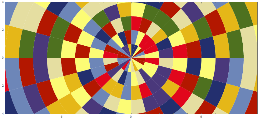
You can use version 10's RandomColor[] instead, if you want it.
An alternative method based on kguler's finding:
ParametricPlot[r {Cos[t], Sin[t]}, {r, 0, 12}, {t, 0, 2 Pi}, Mesh -> 23, Axes -> False, MeshShading -> {{c, c}, {c, c}}, PlotRange -> {{-9, 9}, {-4, 4}}] /. c :> Hue@RandomReal[] 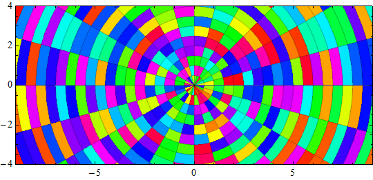
Note that as well as the kguler's answer this is based on undocumented details of the implementation of ParametricPlot and so will not necessarily work in future versions of Mathematica (but it works in v.8.0.4 and 10.0.1).
ParametricPlot[r {Cos[t], Sin[t]}, {t, 0, 2 Pi}, {r, 0, 5}, MeshShading -> {{Red, Blue}, {Yellow, Green}}]? $\endgroup$