4
$\begingroup$

This is a plot of my data

enter image description here

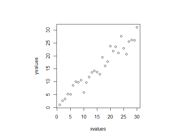
These are the values:

 xvalues yvalues 1 1.091186 2 2.653722 3 3.309146 4 5.206479 5 5.115582 6 8.537005 7 10.013147 8 9.802291 9 10.667769 10 5.809750 11 9.624475 12 11.806013 13 13.587066 14 14.146781 15 13.707472 16 12.891355 17 19.435301 18 16.122108 19 17.768536 20 23.813027 21 21.819081 22 23.556074 23 21.170983 24 27.621148 25 22.932580 26 20.704689 27 25.530339 28 26.227371 29 26.051016 30 31.047145 

I now do a PCA and a biplot of it:

enter image description here

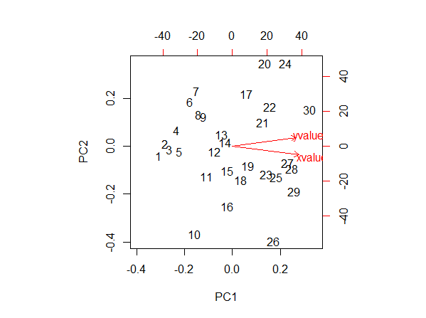
According to Jeromy Anglim in: Interpretation of biplots in principal components analysis in R

The left and bottom axes are showing the loadings; the top and right axes are showing principal component scores.

The left and bottom axes are showing [normalized] principal component scores; the top and right axes are showing the loadings.

I want to be sure I really get this.

Let's start with the loadings: these can be visualized in R by writing:

results <- prcomp(your_data) results$rotation PC1 PC2 xvalues 0.7235616 -0.6902599 yvalues 0.6902599 0.7235616 summary(results) Importance of components: PC1 PC2 Standard deviation 12.0747 1.56606 Proportion of Variance 0.9835 0.01654 Cumulative Proportion 0.9835 1.00000 

Now lets look at the red arrow of xvalues. Its tip is around 0.25 in the x-axis of the loadings. But according to the loadings I have just writen, it should be around 0.72. What am I missing?

Finally, lets look at the point 1. According to the axes, that is telling me the principal component score. Is it that the coordinate in the new frame of reference? It doesn't make sense to me because I think that the new origin of the axes is around the point (15,15) in the Plot 3. If I look at that (and I guess that I am completely wrong here), the point one should have a coordinate around -20 or so, and not 40. Where is my mistake?

Update

I tried plotting this:

plot(pca_results$x) 

enter image description here

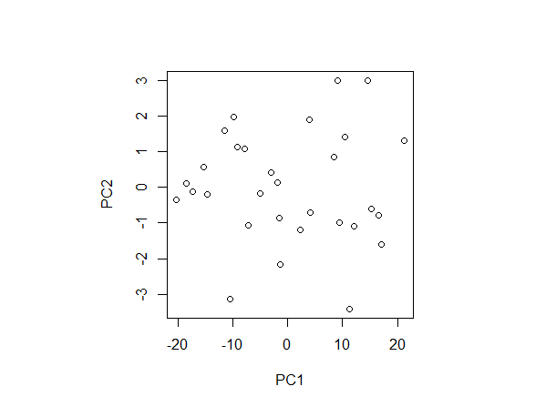
Here it can be seen that the first point has the coordinate that I thought it had to have. But, still, what are the units in the biplot then??

$\endgroup$
6
  • $\begingroup$ Your last paragraph is a bit mystical because it seems to not correspond to your pictures. PCA biplot is can be interpreted as the overlay scatterplot, a superposition of two scatterplots in the same axes (the PCs): plot of the data scores and plot of the variable loadings. You might also want to glance here. $\endgroup$ Commented Dec 25, 2013 at 20:11
  • 2
    $\begingroup$ On your first biplot, the data cloud is round dispite that according to you data PC1 must be much stronger than PC2. This makes me to think that the PC scores on the biplot are standardized (to st. dev. 1). Check if this is true. The loading points (red arrows) are likely to be loadings, as they should. The results$rotation figures you present are clearly the eigenvector values, not the loadings. Please be aware that the R PCA package you use misuses the word "loadings", incorrectly calling eigenvectors "loadings". $\endgroup$ Commented Dec 26, 2013 at 12:22
  • $\begingroup$ How do I check the loadings then? $\endgroup$ Commented Dec 26, 2013 at 12:32
  • $\begingroup$ By definition, "matrix of loadings" (prior rotation or after orthogonal rotation") must have column sum of squares equal to the variances of corresponding factors/components. Thus, in PCA, loadings after extraction and prior rotation are the eigenvectors multiplied by the sq. root of their corresponding eigenvalues (because eigenvalue is the component's variance, prior rotation). $\endgroup$ Commented Dec 26, 2013 at 12:44
  • $\begingroup$ I don't know what your results$rotation matrix actually is. It could be eigenvectors (prior rotation) or it could the orthogonal rotation matrix. Because you didn't show the original data (the values) and full output of your PCA, I can't say. $\endgroup$ Commented Dec 26, 2013 at 12:50

1 Answer 1

6
$\begingroup$

I redid your PCA in SPSS (I'm not R user). It was PCA based on covariances. I confirm your analysis.

Eigenvalues (component variances) and the proportion of overall variance explained I 145.7983424 .9834567 II 2.4525573 .0165433 Eigenvectors (cosines of rotation of variables into components) I II X .7235615578 -.6902598583 Y .6902598583 .7235615578 Loadings (eigenvectors normalized to respective eigenvalues; loadings are the covariances between variables and components) I II X 8.736787614 -1.080991303 Y 8.334679634 1.133143904 Raw componenet scores (Centered XY data multiplied by eigenvectors) I II -20.36311916 -.33895962 -18.56100172 .10137150 -17.38502729 -.11464875 -15.35181292 .56792862 -14.69099392 -.18810082 -11.60576140 1.59724948 -9.86327828 1.97506923 -9.28526215 1.13224207 -7.96429587 1.06820882 -10.59402982 -3.13712683 -7.23731673 -1.06719832 -5.00792706 -.17898115 -3.05497611 .41946048 -1.94506575 .13418887 -1.52474156 -.87393809 -1.36451281 -2.15470883 3.87607199 1.88997907 2.31266941 -1.19757988 4.17269413 -.69654773 9.06852519 2.98675374 8.41574586 .85375121 10.33828396 1.42031271 9.41551294 -.99570731 14.59136448 2.98112427 12.07859576 -1.10160316 11.26433359 -3.40387930 15.31884763 -.60248432 16.52354240 -.78839862 17.12537318 -1.60626218 21.29756203 1.31848485 

The component scores that you plotted as plot(pca_results$x) are these raw component scores printed above.

The component scores on your biplot are these scores scaled to sum-of-squares=1 (sum of squares in each of the 2 columns was brought to 1).

As for the loadings shown as red arrows on the biplot, they are, without doubt, rescaled loadings that I printed above. However - since I'm not R user - I can't tell you how exactly they were rescaled. But I suppose they linearly are related to the true loadings I printed. Biplots can be drawn in multiple ways, with various normalizations. I can't know how your R function exactly does it, and probably it is not too important to know it.

Another my example, even more full, is here. It is the outputs of PCA and LDA (linear discriminant) analyses of iris data.

$\endgroup$
1
  • 1
    $\begingroup$ According to What are the four axes on PCA biplot?, in the default biplot in R the eigenvectors are scaled by the respective standard deviation (square root of the respective eigenvalue) -- this results in loadings -- and then additionally scaled by the square root of the number of observations. $\endgroup$ Commented Jan 14, 2015 at 18:13

Start asking to get answers

Find the answer to your question by asking.

Ask question

Explore related questions

See similar questions with these tags.