12
$\begingroup$

Using a biplot of values obtained through principal component analysis, it is possible to explore the explanatory variables that make up each principle component. Is this also possible with Linear Discriminant Analysis?

Examples provided use the The data is "Edgar Anderson's Iris Data" (http://en.wikipedia.org/wiki/Iris_flower_data_set). Here is the iris data:

 id SLength SWidth PLength PWidth species 1 5.1 3.5 1.4 .2 setosa 2 4.9 3.0 1.4 .2 setosa 3 4.7 3.2 1.3 .2 setosa 4 4.6 3.1 1.5 .2 setosa 5 5.0 3.6 1.4 .2 setosa 6 5.4 3.9 1.7 .4 setosa 7 4.6 3.4 1.4 .3 setosa 8 5.0 3.4 1.5 .2 setosa 9 4.4 2.9 1.4 .2 setosa 10 4.9 3.1 1.5 .1 setosa 11 5.4 3.7 1.5 .2 setosa 12 4.8 3.4 1.6 .2 setosa 13 4.8 3.0 1.4 .1 setosa 14 4.3 3.0 1.1 .1 setosa 15 5.8 4.0 1.2 .2 setosa 16 5.7 4.4 1.5 .4 setosa 17 5.4 3.9 1.3 .4 setosa 18 5.1 3.5 1.4 .3 setosa 19 5.7 3.8 1.7 .3 setosa 20 5.1 3.8 1.5 .3 setosa 21 5.4 3.4 1.7 .2 setosa 22 5.1 3.7 1.5 .4 setosa 23 4.6 3.6 1.0 .2 setosa 24 5.1 3.3 1.7 .5 setosa 25 4.8 3.4 1.9 .2 setosa 26 5.0 3.0 1.6 .2 setosa 27 5.0 3.4 1.6 .4 setosa 28 5.2 3.5 1.5 .2 setosa 29 5.2 3.4 1.4 .2 setosa 30 4.7 3.2 1.6 .2 setosa 31 4.8 3.1 1.6 .2 setosa 32 5.4 3.4 1.5 .4 setosa 33 5.2 4.1 1.5 .1 setosa 34 5.5 4.2 1.4 .2 setosa 35 4.9 3.1 1.5 .2 setosa 36 5.0 3.2 1.2 .2 setosa 37 5.5 3.5 1.3 .2 setosa 38 4.9 3.6 1.4 .1 setosa 39 4.4 3.0 1.3 .2 setosa 40 5.1 3.4 1.5 .2 setosa 41 5.0 3.5 1.3 .3 setosa 42 4.5 2.3 1.3 .3 setosa 43 4.4 3.2 1.3 .2 setosa 44 5.0 3.5 1.6 .6 setosa 45 5.1 3.8 1.9 .4 setosa 46 4.8 3.0 1.4 .3 setosa 47 5.1 3.8 1.6 .2 setosa 48 4.6 3.2 1.4 .2 setosa 49 5.3 3.7 1.5 .2 setosa 50 5.0 3.3 1.4 .2 setosa 51 7.0 3.2 4.7 1.4 versicolor 52 6.4 3.2 4.5 1.5 versicolor 53 6.9 3.1 4.9 1.5 versicolor 54 5.5 2.3 4.0 1.3 versicolor 55 6.5 2.8 4.6 1.5 versicolor 56 5.7 2.8 4.5 1.3 versicolor 57 6.3 3.3 4.7 1.6 versicolor 58 4.9 2.4 3.3 1.0 versicolor 59 6.6 2.9 4.6 1.3 versicolor 60 5.2 2.7 3.9 1.4 versicolor 61 5.0 2.0 3.5 1.0 versicolor 62 5.9 3.0 4.2 1.5 versicolor 63 6.0 2.2 4.0 1.0 versicolor 64 6.1 2.9 4.7 1.4 versicolor 65 5.6 2.9 3.6 1.3 versicolor 66 6.7 3.1 4.4 1.4 versicolor 67 5.6 3.0 4.5 1.5 versicolor 68 5.8 2.7 4.1 1.0 versicolor 69 6.2 2.2 4.5 1.5 versicolor 70 5.6 2.5 3.9 1.1 versicolor 71 5.9 3.2 4.8 1.8 versicolor 72 6.1 2.8 4.0 1.3 versicolor 73 6.3 2.5 4.9 1.5 versicolor 74 6.1 2.8 4.7 1.2 versicolor 75 6.4 2.9 4.3 1.3 versicolor 76 6.6 3.0 4.4 1.4 versicolor 77 6.8 2.8 4.8 1.4 versicolor 78 6.7 3.0 5.0 1.7 versicolor 79 6.0 2.9 4.5 1.5 versicolor 80 5.7 2.6 3.5 1.0 versicolor 81 5.5 2.4 3.8 1.1 versicolor 82 5.5 2.4 3.7 1.0 versicolor 83 5.8 2.7 3.9 1.2 versicolor 84 6.0 2.7 5.1 1.6 versicolor 85 5.4 3.0 4.5 1.5 versicolor 86 6.0 3.4 4.5 1.6 versicolor 87 6.7 3.1 4.7 1.5 versicolor 88 6.3 2.3 4.4 1.3 versicolor 89 5.6 3.0 4.1 1.3 versicolor 90 5.5 2.5 4.0 1.3 versicolor 91 5.5 2.6 4.4 1.2 versicolor 92 6.1 3.0 4.6 1.4 versicolor 93 5.8 2.6 4.0 1.2 versicolor 94 5.0 2.3 3.3 1.0 versicolor 95 5.6 2.7 4.2 1.3 versicolor 96 5.7 3.0 4.2 1.2 versicolor 97 5.7 2.9 4.2 1.3 versicolor 98 6.2 2.9 4.3 1.3 versicolor 99 5.1 2.5 3.0 1.1 versicolor 100 5.7 2.8 4.1 1.3 versicolor 101 6.3 3.3 6.0 2.5 virginica 102 5.8 2.7 5.1 1.9 virginica 103 7.1 3.0 5.9 2.1 virginica 104 6.3 2.9 5.6 1.8 virginica 105 6.5 3.0 5.8 2.2 virginica 106 7.6 3.0 6.6 2.1 virginica 107 4.9 2.5 4.5 1.7 virginica 108 7.3 2.9 6.3 1.8 virginica 109 6.7 2.5 5.8 1.8 virginica 110 7.2 3.6 6.1 2.5 virginica 111 6.5 3.2 5.1 2.0 virginica 112 6.4 2.7 5.3 1.9 virginica 113 6.8 3.0 5.5 2.1 virginica 114 5.7 2.5 5.0 2.0 virginica 115 5.8 2.8 5.1 2.4 virginica 116 6.4 3.2 5.3 2.3 virginica 117 6.5 3.0 5.5 1.8 virginica 118 7.7 3.8 6.7 2.2 virginica 119 7.7 2.6 6.9 2.3 virginica 120 6.0 2.2 5.0 1.5 virginica 121 6.9 3.2 5.7 2.3 virginica 122 5.6 2.8 4.9 2.0 virginica 123 7.7 2.8 6.7 2.0 virginica 124 6.3 2.7 4.9 1.8 virginica 125 6.7 3.3 5.7 2.1 virginica 126 7.2 3.2 6.0 1.8 virginica 127 6.2 2.8 4.8 1.8 virginica 128 6.1 3.0 4.9 1.8 virginica 129 6.4 2.8 5.6 2.1 virginica 130 7.2 3.0 5.8 1.6 virginica 131 7.4 2.8 6.1 1.9 virginica 132 7.9 3.8 6.4 2.0 virginica 133 6.4 2.8 5.6 2.2 virginica 134 6.3 2.8 5.1 1.5 virginica 135 6.1 2.6 5.6 1.4 virginica 136 7.7 3.0 6.1 2.3 virginica 137 6.3 3.4 5.6 2.4 virginica 138 6.4 3.1 5.5 1.8 virginica 139 6.0 3.0 4.8 1.8 virginica 140 6.9 3.1 5.4 2.1 virginica 141 6.7 3.1 5.6 2.4 virginica 142 6.9 3.1 5.1 2.3 virginica 143 5.8 2.7 5.1 1.9 virginica 144 6.8 3.2 5.9 2.3 virginica 145 6.7 3.3 5.7 2.5 virginica 146 6.7 3.0 5.2 2.3 virginica 147 6.3 2.5 5.0 1.9 virginica 148 6.5 3.0 5.2 2.0 virginica 149 6.2 3.4 5.4 2.3 virginica 150 5.9 3.0 5.1 1.8 virginica 

Example PCA biplot using the iris data set in R (code below):

enter image description here

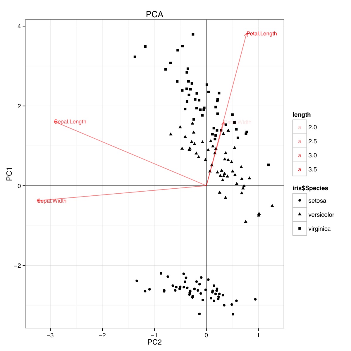
This figure indicates that Petal length and Petal width are important in determining PC1 score and in discriminating between Species groups. setosa has smaller petals and wider sepals.

Apparently, similar conclusions can be drawn from plotting linear discriminant analysis results, though I am not certain what the LDA plot presents, hence the question. The axis are the two first linear discriminants (LD1 99% and LD2 1% of trace). The coordinates of the red vectors are "Coefficients of linear discriminants" also described as "scaling" (lda.fit$scaling: a matrix which transforms observations to discriminant functions, normalized so that within groups covariance matrix is spherical). "scaling" is calculated as diag(1/f1, , p) and f1 is sqrt(diag(var(x - group.means[g, ]))). Data can be projected onto the linear discriminants (using predict.lda) (code below, as demonstrated https://stackoverflow.com/a/17240647/742447). The data and the predictor variables are plotted together so that which species are defined by an increase in which predictor variables can be seen (as is done for usual PCA biplots and the above PCA biplot).:

Example LDA biplot using the iris data set in R

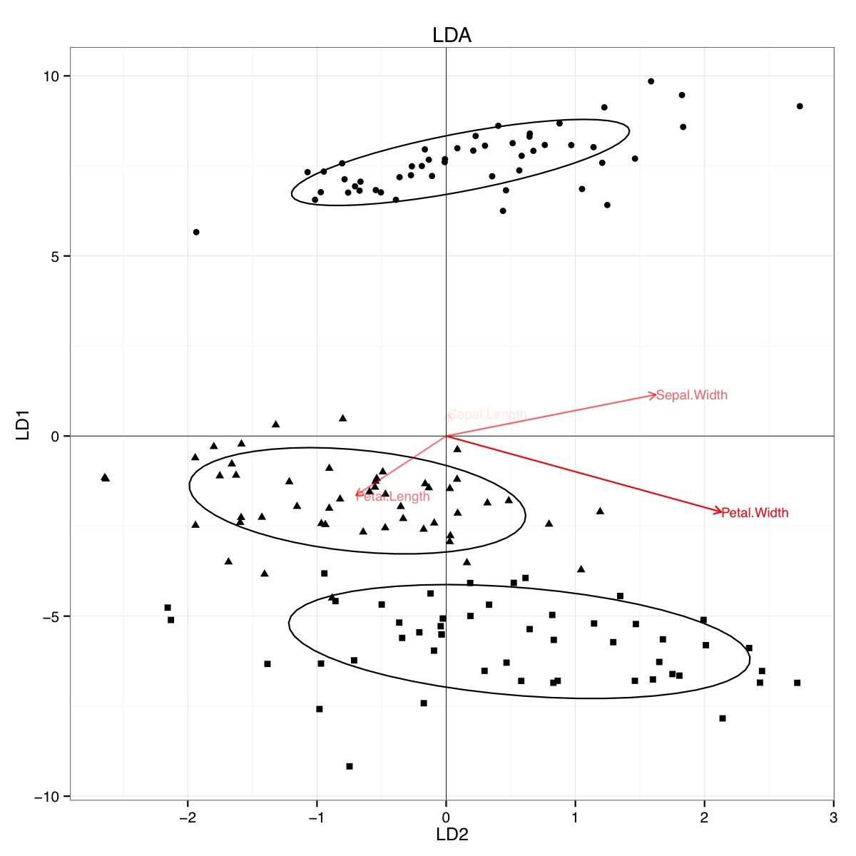
From this plot, Sepal width, Petal Width and Petal Length all contribute to a similar level to LD1. As expected, setosa appears to smaller petals and wider sepals.

There is no built-in way to plot such biplots from LDA in R and few discussions of this online, which makes me wary of this approach.

Does this LDA plot (see code below) provide a statistically valid interpretation of predictor variable scaling scores ?

Code for PCA:

require(grid) iris.pca <- prcomp(iris[,-5]) PC <- iris.pca x="PC1" y="PC2" PCdata <- data.frame(obsnames=iris[,5], PC$x) datapc <- data.frame(varnames=rownames(PC$rotation), PC$rotation) mult <- min( (max(PCdata[,y]) - min(PCdata[,y])/(max(datapc[,y])-min(datapc[,y]))), (max(PCdata[,x]) - min(PCdata[,x])/(max(datapc[,x])-min(datapc[,x]))) ) datapc <- transform(datapc, v1 = 1.6 * mult * (get(x)), v2 = 1.6 * mult * (get(y)) ) datapc$length <- with(datapc, sqrt(v1^2+v2^2)) datapc <- datapc[order(-datapc$length),] p <- qplot(data=data.frame(iris.pca$x), main="PCA", x=PC1, y=PC2, shape=iris$Species) #p <- p + stat_ellipse(aes(group=iris$Species)) p <- p + geom_hline(aes(0), size=.2) + geom_vline(aes(0), size=.2) p <- p + geom_text(data=datapc, aes(x=v1, y=v2, label=varnames, shape=NULL, linetype=NULL, alpha=length), size = 3, vjust=0.5, hjust=0, color="red") p <- p + geom_segment(data=datapc, aes(x=0, y=0, xend=v1, yend=v2, shape=NULL, linetype=NULL, alpha=length), arrow=arrow(length=unit(0.2,"cm")), alpha=0.5, color="red") p <- p + coord_flip() print(p) 

Code for LDA

#Perform LDA analysis iris.lda <- lda(as.factor(Species)~., data=iris) #Project data on linear discriminants iris.lda.values <- predict(iris.lda, iris[,-5]) #Extract scaling for each predictor and data.lda <- data.frame(varnames=rownames(coef(iris.lda)), coef(iris.lda)) #coef(iris.lda) is equivalent to iris.lda$scaling data.lda$length <- with(data.lda, sqrt(LD1^2+LD2^2)) scale.para <- 0.75 #Plot the results p <- qplot(data=data.frame(iris.lda.values$x), main="LDA", x=LD1, y=LD2, shape=iris$Species)#+stat_ellipse() p <- p + geom_hline(aes(0), size=.2) + geom_vline(aes(0), size=.2) p <- p + theme(legend.position="none") p <- p + geom_text(data=data.lda, aes(x=LD1*scale.para, y=LD2*scale.para, label=varnames, shape=NULL, linetype=NULL, alpha=length), size = 3, vjust=0.5, hjust=0, color="red") p <- p + geom_segment(data=data.lda, aes(x=0, y=0, xend=LD1*scale.para, yend=LD2*scale.para, shape=NULL, linetype=NULL, alpha=length), arrow=arrow(length=unit(0.2,"cm")), color="red") p <- p + coord_flip() print(p) 

The results of the LDA are as follows

lda(as.factor(Species) ~ ., data = iris) Prior probabilities of groups: setosa versicolor virginica 0.3333333 0.3333333 0.3333333 Group means: Sepal.Length Sepal.Width Petal.Length Petal.Width setosa 5.006 3.428 1.462 0.246 versicolor 5.936 2.770 4.260 1.326 virginica 6.588 2.974 5.552 2.026 Coefficients of linear discriminants: LD1 LD2 Sepal.Length 0.8293776 0.02410215 Sepal.Width 1.5344731 2.16452123 Petal.Length -2.2012117 -0.93192121 Petal.Width -2.8104603 2.83918785 Proportion of trace: LD1 LD2 0.9912 0.0088 
$\endgroup$
4
  • $\begingroup$ I can't follow your code (I'm not R user and I'd prefer to see actual data and results values rather than unexplained pictures and unexplained code), sorry. What do your plots plot? What are the coordinates of the red vectors - regressional weights of the latents or of the variables? What did you plot as well data poins for? What is discriminant predictor variable scaling scores? - the term seems to me not common and strange. $\endgroup$ Commented Jan 21, 2014 at 14:22
  • $\begingroup$ @ttnphns: thank you for suggesting question improvements which are now reflected in the question. $\endgroup$ Commented Jan 22, 2014 at 14:01
  • $\begingroup$ I still don't know what is predictor variable scaling scores. Maybe "discriminant scores"? Anyway, I added an answer which might be of your interest. $\endgroup$ Commented Jan 23, 2014 at 14:03
  • $\begingroup$ How can you perform in a similar way when you just have two classes in the classifier variable? $\endgroup$ Commented Jan 17, 2024 at 10:55

3 Answers 3

11
+100
$\begingroup$

Principal components analysis and Linear discriminant analysis outputs; iris data.

I will not be drawing biplots because biplots can drawn with various normalizations and therefore may look different. Since I'm not R user I have difficulty to track down how you produced your plots, to repeat them. Instead, I will do PCA and LDA and show the results, in a manner similar to this (you might want to read). Both analyses done in SPSS.

Principal components of iris data:

The analysis will be based on covariances (not correlations) between the 4 variables. Eigenvalues (component variances) and the proportion of overall variance explained PC1 4.228241706 .924618723 PC2 .242670748 .053066483 PC3 .078209500 .017102610 PC4 .023835093 .005212184 # @Etienne's comment: # Eigenvalues are obtained in R by # (princomp(iris[,-5])$sdev)^2 or (prcomp(iris[,-5])$sdev)^2. # Proportion of variance explained is obtained in R by # summary(princomp(iris[,-5])) or summary(prcomp(iris[,-5])) Eigenvectors (cosines of rotation of variables into components) PC1 PC2 PC3 PC4 SLength .3613865918 .6565887713 -.5820298513 .3154871929 SWidth -.0845225141 .7301614348 .5979108301 -.3197231037 PLength .8566706060 -.1733726628 .0762360758 -.4798389870 PWidth .3582891972 -.0754810199 .5458314320 .7536574253 # @Etienne's comment: # This is obtained in R by # prcomp(iris[,-5])$rotation or princomp(iris[,-5])$loadings Loadings (eigenvectors normalized to respective eigenvalues; loadings are the covariances between variables and standardized components) PC1 PC2 PC3 PC4 SLength .743108002 .323446284 -.162770244 .048706863 SWidth -.173801015 .359689372 .167211512 -.049360829 PLength 1.761545107 -.085406187 .021320152 -.074080509 PWidth .736738926 -.037183175 .152647008 .116354292 # @Etienne's comment: # Loadings can be obtained in R with # t(t(princomp(iris[,-5])$loadings) * princomp(iris[,-5])$sdev) or # t(t(prcomp(iris[,-5])$rotation) * prcomp(iris[,-5])$sdev) Standardized (rescaled) loadings (loadings divided by st. deviations of the respective variables) PC1 PC2 PC3 PC4 SLength .897401762 .390604412 -.196566721 .058820016 SWidth -.398748472 .825228709 .383630296 -.113247642 PLength .997873942 -.048380599 .012077365 -.041964868 PWidth .966547516 -.048781602 .200261695 .152648309 Raw component scores (Centered 4-variable data multiplied by eigenvectors) PC1 PC2 PC3 PC4 -2.684125626 .319397247 -.027914828 .002262437 -2.714141687 -.177001225 -.210464272 .099026550 -2.888990569 -.144949426 .017900256 .019968390 -2.745342856 -.318298979 .031559374 -.075575817 -2.728716537 .326754513 .090079241 -.061258593 -2.280859633 .741330449 .168677658 -.024200858 -2.820537751 -.089461385 .257892158 -.048143106 -2.626144973 .163384960 -.021879318 -.045297871 -2.886382732 -.578311754 .020759570 -.026744736 -2.672755798 -.113774246 -.197632725 -.056295401 ... etc. # @Etienne's comment: # This is obtained in R with # prcomp(iris[,-5])$x or princomp(iris[,-5])$scores. # Can also be eigenvector normalized for plotting Standardized (to unit variances) component scores, when multiplied by loadings return original centered variables. 

It is important to stress that it is loadings, not eigenvectors, by which we typically interpret principal components (or factors in factor analysis) - if we need to interpret. Loadings are the regressional coefficients of modeling variables by standardized components. At the same time, because components don't intercorrelate, they are the covariances between such components and the variables. Standardized (rescaled) loadings, like correlations, cannot exceed 1, and are more handy to interpret because the effect of unequal variances of variables is taken off.

It is loadings, not eigenvectors, that are typically displayed on a biplot side-by-side with component scores; the latter are often displayed column-normalized.


Linear discriminants of iris data:

There is 3 classes and 4 variables: min(3-1,4)=2 discriminants can be extracted. Only the extraction (no classification of data points) will be done. The Within scatter matrix 38.95620000 13.63000000 24.62460000 5.64500000 13.63000000 16.96200000 8.12080000 4.80840000 24.62460000 8.12080000 27.22260000 6.27180000 5.64500000 4.80840000 6.27180000 6.15660000 The Between scatter matrix 63.2121333 -19.9526667 165.2484000 71.2793333 -19.9526667 11.3449333 -57.2396000 -22.9326667 165.2484000 -57.2396000 437.1028000 186.7740000 71.2793333 -22.9326667 186.7740000 80.4133333 Eigenvalues and canonical correlations (Canonical correlation squared is SSbetween/SStotal of ANOVA by that discriminant) Dis1 32.19192920 .98482089 Dis2 .28539104 .47119702 # @Etienne's comment: # In R eigenvalues are expected from # lda(as.factor(Species)~.,data=iris)$svd, but this produces # Dis1 Dis2 # 48.642644 4.579983 # @ttnphns' comment: # The difference might be due to different computational approach # (e.g. me used eigendecomposition and R used svd?) and is of no importance. # Canonical correlations though should be the same. Eigenvectors Dis1 Dis2 SLength -.0684059150 .0019879117 SWidth -.1265612055 .1785267025 PLength .1815528774 -.0768635659 PWidth .2318028594 .2341722673 Eigenvectors (as before, but column-normalized to SS=1: cosines of rotation of variables into discriminants). Dis1 Dis2 SLength -.2087418215 .0065319640 SWidth -.3862036868 .5866105531 PLength .5540117156 -.2525615400 PWidth .7073503964 .7694530921 Unstandardized discriminant coefficients (proportionally related to eigenvectors) Dis1 Dis2 SLength -.829377642 .024102149 SWidth -1.534473068 2.164521235 PLength 2.201211656 -.931921210 PWidth 2.810460309 2.839187853 # @Etienne's comment: # This is obtained in R with # lda(as.factor(Species)~.,data=iris)$scaling # which is described as being standardized discriminant coefficients in the function definition. Standardized discriminant coefficients Dis1 Dis2 SLength -.4269548486 .0124075316 SWidth -.5212416758 .7352613085 PLength .9472572487 -.4010378190 PWidth .5751607719 .5810398645 Pooled within-groups correlations between variables and discriminants Dis1 Dis2 SLength .2225959415 .3108117231 SWidth -.1190115149 .8636809224 PLength .7060653811 .1677013843 PWidth .6331779262 .7372420588 Discriminant scores (Centered 4-variable data multiplied by unstandardized coefficients) Dis1 Dis2 -8.061799783 .300420621 -7.128687721 -.786660426 -7.489827971 -.265384488 -6.813200569 -.670631068 -8.132309326 .514462530 -7.701946744 1.461720967 -7.212617624 .355836209 -7.605293546 -.011633838 -6.560551593 -1.015163624 -7.343059893 -.947319209 ... etc. # @Etienne's comment: # This is obtained in R with # predict(lda(as.factor(Species)~.,data=iris), iris[,-5])$x 

About computations at extraction of discriminants in LDA please look here. We interpret discriminants usually by discriminant coefficients or standardized discriminant coefficients (the latter are more handy because differential variance in variables is taken off). This is like in PCA. But, note: the coefficients here are the regressional coefficients of modeling discriminants by variables, not vice versa, like it was in PCA. Because variables are not uncorrelated, the coefficients cannot be seen as covariances between variables and discriminants.

Yet we have another matrix instead which may serve as an alternative source of interpretation of discriminants - pooled within-group correlations between the discriminants and the variables. Because discriminants are uncorrelated, like PCs, this matrix is in a sense analogous to the standardized loadings of PCA.

In all, while in PCA we have the only matrix - loadings - to help interpret the latents, in LDA we have two alternative matrices for that. If you need to plot (biplot or whatever), you have to decide whether to plot coefficients or correlations.

And, of course, needless to remind that in PCA of iris data the components don't "know" that there are 3 classes; they can't be expected to discriminate classes. Discriminants do "know" there are classes and it is their natural job which is to discriminate.

$\endgroup$
13
  • $\begingroup$ So I can plot, after arbitrary scaling, either "Standardized discriminant coefficients" or "Pooled within-groups correlations between variables and discriminants" on the same axis as "Discriminant scores" to interpret the results in two different ways? In my question I had plotted "Unstandardized discriminant coefficients" on the same axis as the "Discriminant scores". $\endgroup$ Commented Jan 24, 2014 at 14:46
  • 1
    $\begingroup$ @Etienne I added details you asked for to the bottom of this answer stats.stackexchange.com/a/48859/3277. Thank you for your generosity. $\endgroup$ Commented Jan 24, 2014 at 16:56
  • 1
    $\begingroup$ @TLJ, should be: between variables and standardized components. I've inserted the word. See please here: Loadings are the coefficients to predict... as well as here: [Footnote: The components' values...]. Loadings are coefficients to compute variables from standardized and orthogonal components, by virtue of what loadings are the covariances between these and those. $\endgroup$ Commented Aug 18, 2014 at 17:46
  • 1
    $\begingroup$ @TLJ, "these and those" = variables and components. You said you computed raw component scores. Standardize each component to variance=1. Compute covariances between the variables and the components. That would be the loadings. "Standardized" or "rescaled" loading is the loading divided by the st. deviation of the respective variable. $\endgroup$ Commented Aug 18, 2014 at 20:33
  • 1
    $\begingroup$ Loading squared is the share of the variable's variance that is accounted for by the component. $\endgroup$ Commented Aug 18, 2014 at 22:41
5
$\begingroup$

My understanding is that biplots of linear discriminant analyses can be done, it is implemented in fact in R packages ggbiplot and ggord and another function to do it is posted in this StackOverflow thread.

Also the book "Biplots in practice" by M. Greenacre has one chapter (chapter 11, see pdf) on it and in Figure 11.5 it shows a biplot of a linear discriminant analysis of the iris dataset: enter image description here

$\endgroup$
2
  • 1
    $\begingroup$ Actually, the whole book is freely available online (one pdf per chapter) here multivariatestatistics.org/biplots.html. $\endgroup$ Commented Aug 6, 2015 at 16:36
  • $\begingroup$ Aha no dodgy websites needed even, thanks for that! $\endgroup$ Commented Aug 6, 2015 at 16:51
3
$\begingroup$

I know this was asked over a year ago, and ttnphns gave an excellent and in-depth answer, but I thought I'd add a couple of comments for those (like me) that are interested in PCA and LDA for their usefulness in ecological sciences, but have limited statistical background (not statisticians).

PCs in PCA are linear combinations of original variables that sequentially maximally explain total variance in the multidimensional dataset. You will have as many PCs as you do original variables. The percent of the variance the PCs explain is given by the eigenvalues of the similarity matrix used, and the coefficient for each original variable on each new PC is given by the eigenvectors. PCA has no assumptions about groups. PCA is very good for seeing how multiple variables change in value across your data (in a biplot, for example). Interpreting a PCA relies heavily on the biplot.

LDA is different for a very important reason - it creates new variables (LDs) by maximizing variance between groups. These are still linear combinations of original variables, but rather than explain as much variance as possible with each sequential LD, instead they are drawn to maximize the DIFFERENCE between groups along that new variable. Rather than a similarity matrix, LDA (and MANOVA) use a comparison matrix of between and within groups sum of squares and cross-products. The eigenvectors of this matrix - the coefficients that the OP was originally concerned with - describe how much the original variables contribute to the formation of the new LDs.

For these reasons, the eigenvectors from the PCA will give you a better idea how a variable changes in value across your data cloud, and how important it is to total variance in your dataset, than the LDA. However, the LDA, particularly in combination with a MANOVA, will give you a statistical test of difference in multivariate centroids of your groups, and an estimate of error in allocation of points to their respective groups (in a sense, multivariate effect size). In an LDA, even if a variable changes linearly (and significantly) across groups, its coefficient on an LD may not indicate the "scale" of that effect, and depends entirely on the other variables included in the analysis.

I hope that was clear. Thanks for your time. See a picture below...

PCs and LDs are constructed differently, and coefficients for an LD may not give you a sense of how original variables vary in your dataset

$\endgroup$
2
  • 1
    $\begingroup$ This is all correct, and +1 from me, but I am not sure how your answer addresses the original question, which was very specifically about how to draw a LDA biplot. $\endgroup$ Commented Feb 6, 2015 at 17:51
  • $\begingroup$ I suppose you're right - I was responding to this, mostly "Using a biplot of values obtained through principal component analysis, it is possible to explore the explanatory variables that make up each principle component. Is this also possible with Linear Discriminant Analysis?" - and the answer is, yes, but the meaning is very different, as described above... Thanks for the comment and +1! $\endgroup$ Commented Feb 10, 2015 at 15:31

Start asking to get answers

Find the answer to your question by asking.

Ask question

Explore related questions

See similar questions with these tags.