(In your example spreadsheet you have no formulas)
Most likely your formula calculated results are given in TEXT format, so AVERAGE -which needs numbers to make calculations- can NOT give any results and you end up with #DIV/0!.
A quick and easy fix:
To change text cells to number cells, select your range (C2:C) and choose a number format for it by going to the top menu, Format --> Number.
Your other alternative is to use the function VALUE within the Arrayformula so as to get the results formatted as numbers.
EDIT (following OP's sharing the sheet)
Your problem lies on rows 1496-1499.
In your buys sheet, rows 1496-1499, in column M (Price) the value is 0.
This causes your formula =ARRAYFORMULA(1- B2:B3796/A2:A3796) for Profit margin in Sheet1in column Cto give #DIV/0! which in turn gives #DIV/0! in column E (Average margin).
To solve this (as mentioned above):
- Change your formula for
Average margin to =IFERROR(average(C2:C), "CHECK your buys") - Check your buys
Extra tip: As an additional step, use conditional formatting in your buys sheet, to easily spot the issues.