Artificial Intelligence, Machine Learning and Deep Learning

AI, Machine Learning and Deep Learning Sujit Pal, Abhishek Sharma

Outline • Artificial Intelligence • AI vs ML vs DL • Machine Learning o Example – Character recognition o Another Example o General Flow o Need for Deep Learning • Deep Learning • Learn more ? • References Footer Text 2

Artificial Intelligence • “ [The automation of] activities that we associate with human thinking, activities such as decision-making, problem solving, learning ..."(Bellman, 1978) • "A field of study that seeks to explain and emulate intelligent behavior in terms of computational processes" (Schalkoff, 1 990) • “The capability of a machine to immitate intellignet human behavior”. (merriam-webster) Footer Text 3

Artificial Intelligence • Examples: o Movie/ Songs recommendation o Fraud Detection – credit card purchases o Smart home devices o Facebook – tagging friends o Video Games o Virtual Personal Assistants: Siri, Cortana Footer Text 4

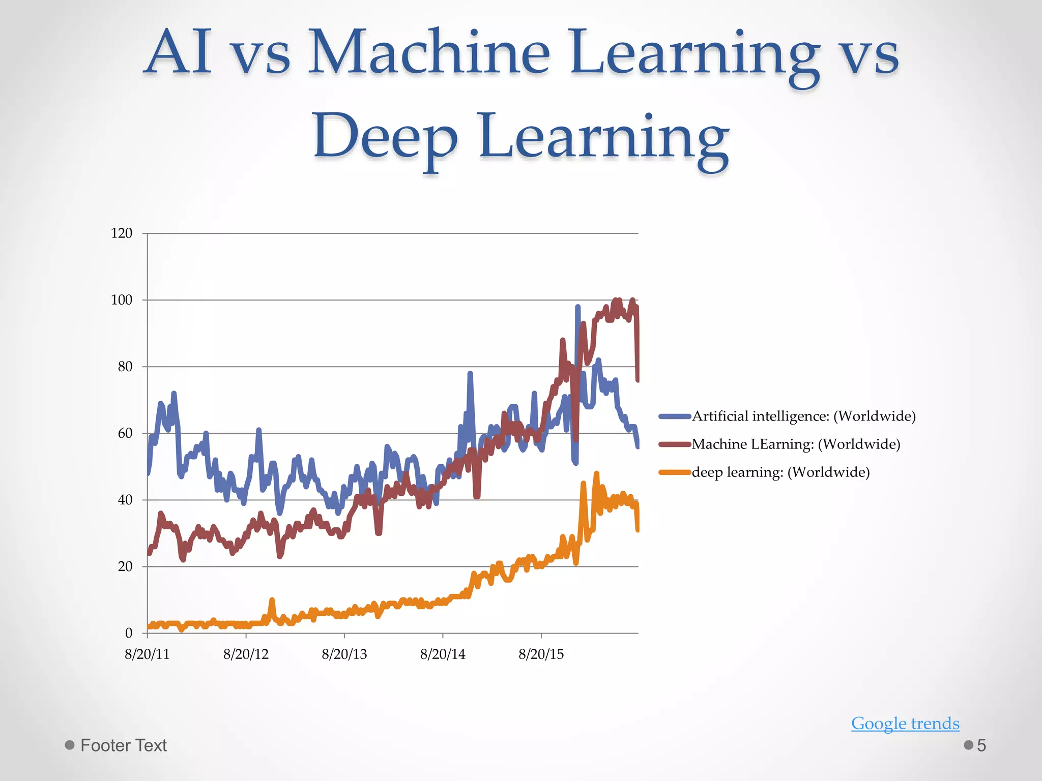
AI vs Machine Learning vs Deep Learning 0 20 40 60 80 100 120 8/20/11 8/20/12 8/20/13 8/20/14 8/20/15 Artificial intelligence: (Worldwide) Machine LEarning: (Worldwide) deep learning: (Worldwide) Google trends Footer Text 5

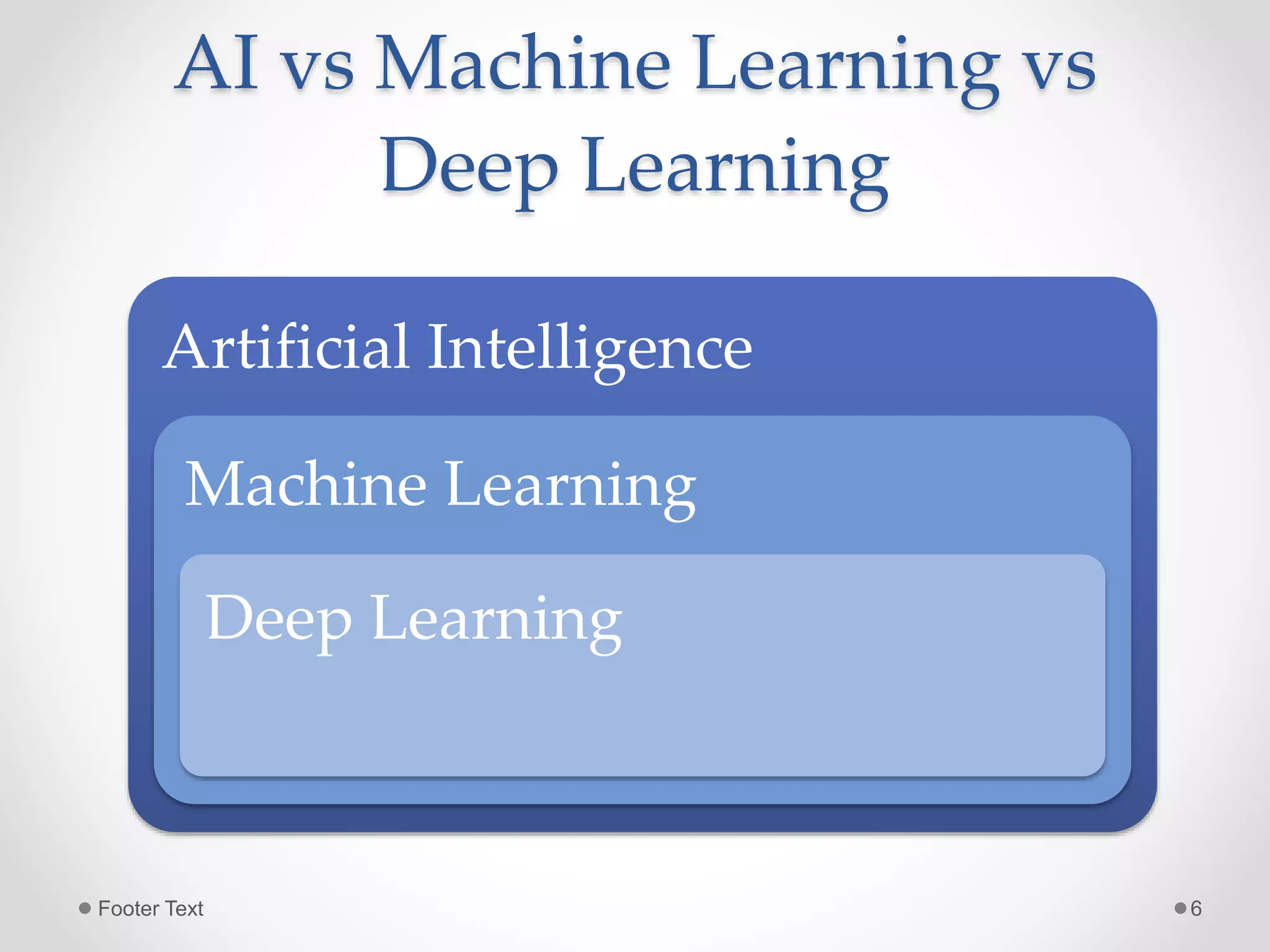
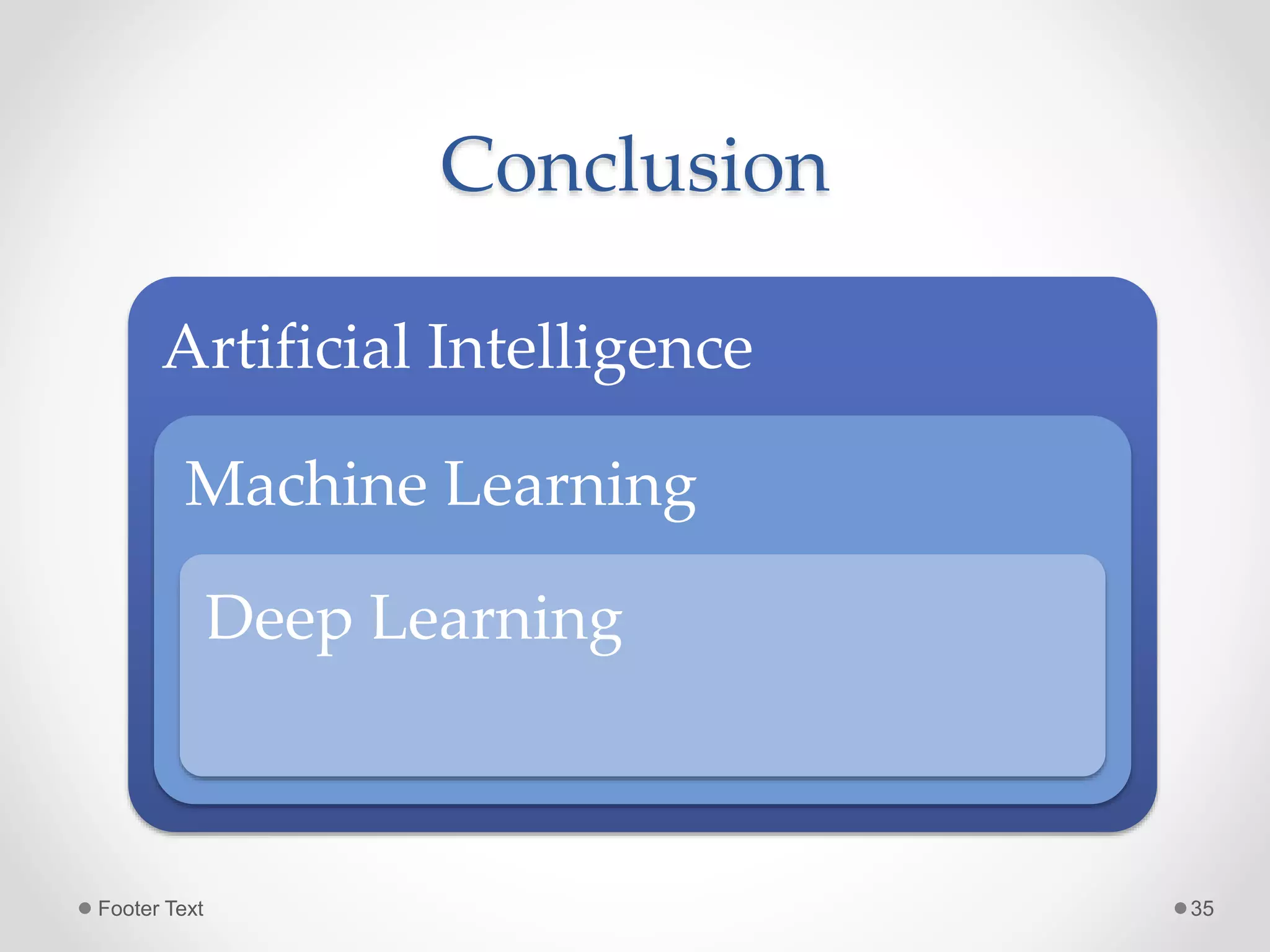
AI vs Machine Learning vs Deep Learning Artificial Intelligence Machine Learning Deep Learning Footer Text 6

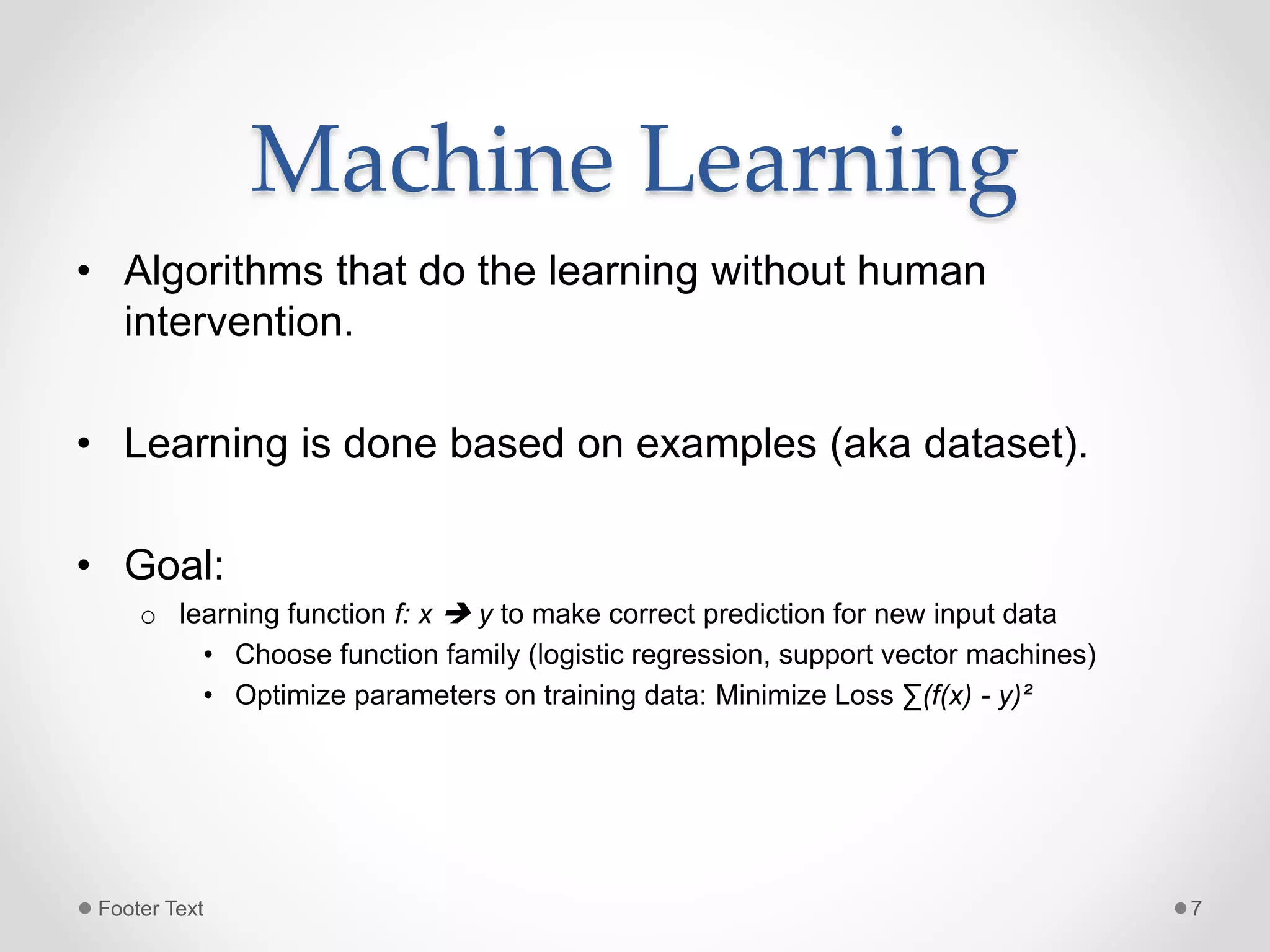
Machine Learning • Algorithms that do the learning without human intervention. • Learning is done based on examples (aka dataset). • Goal: o learning function f: x  y to make correct prediction for new input data • Choose function family (logistic regression, support vector machines) • Optimize parameters on training data: Minimize Loss ∑(f(x) - y)² Footer Text 7

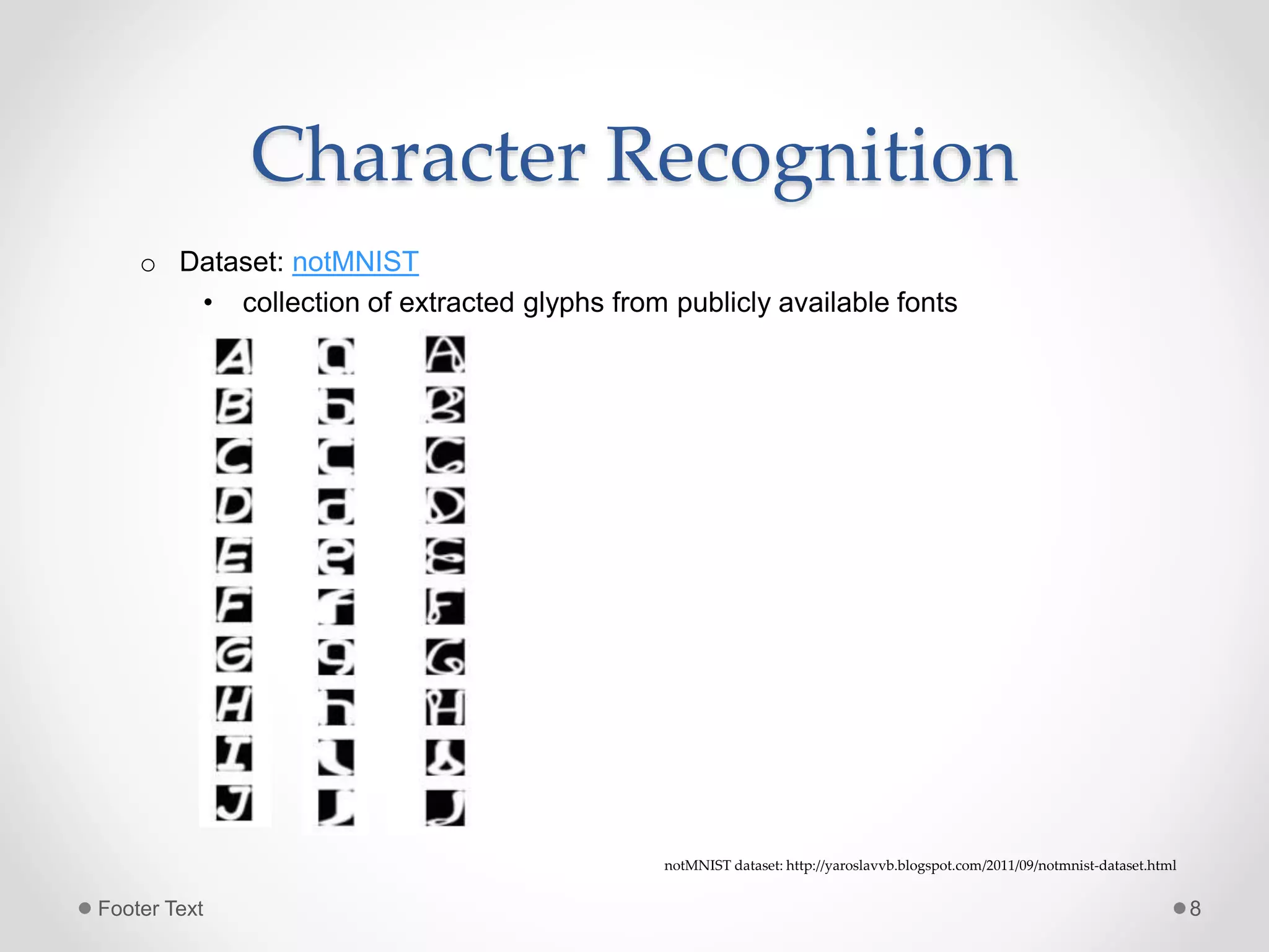
Character Recognition o Dataset: notMNIST • collection of extracted glyphs from publicly available fonts notMNIST dataset: http://yaroslavvb.blogspot.com/2011/09/notmnist-dataset.html Footer Text 8

Character Recognition function = LogisticRegression() features_testset = test_dataset.reshape(test_dataset.shape[0], 28 * 28) labels_testset = test_labels feature_trainingset = train_dataset[:sample_size].reshape(sample_size, 28*28) labels_traininigset = train_labels[:sample_size] function.fit(feature_trainingset, labels_traininigset) function.score(features_testset, labels_testset) Accuracy: 0.856199 prepare model; learn weights prediction/ inference evaluation *Library: Scikit-learn Footer Text 9

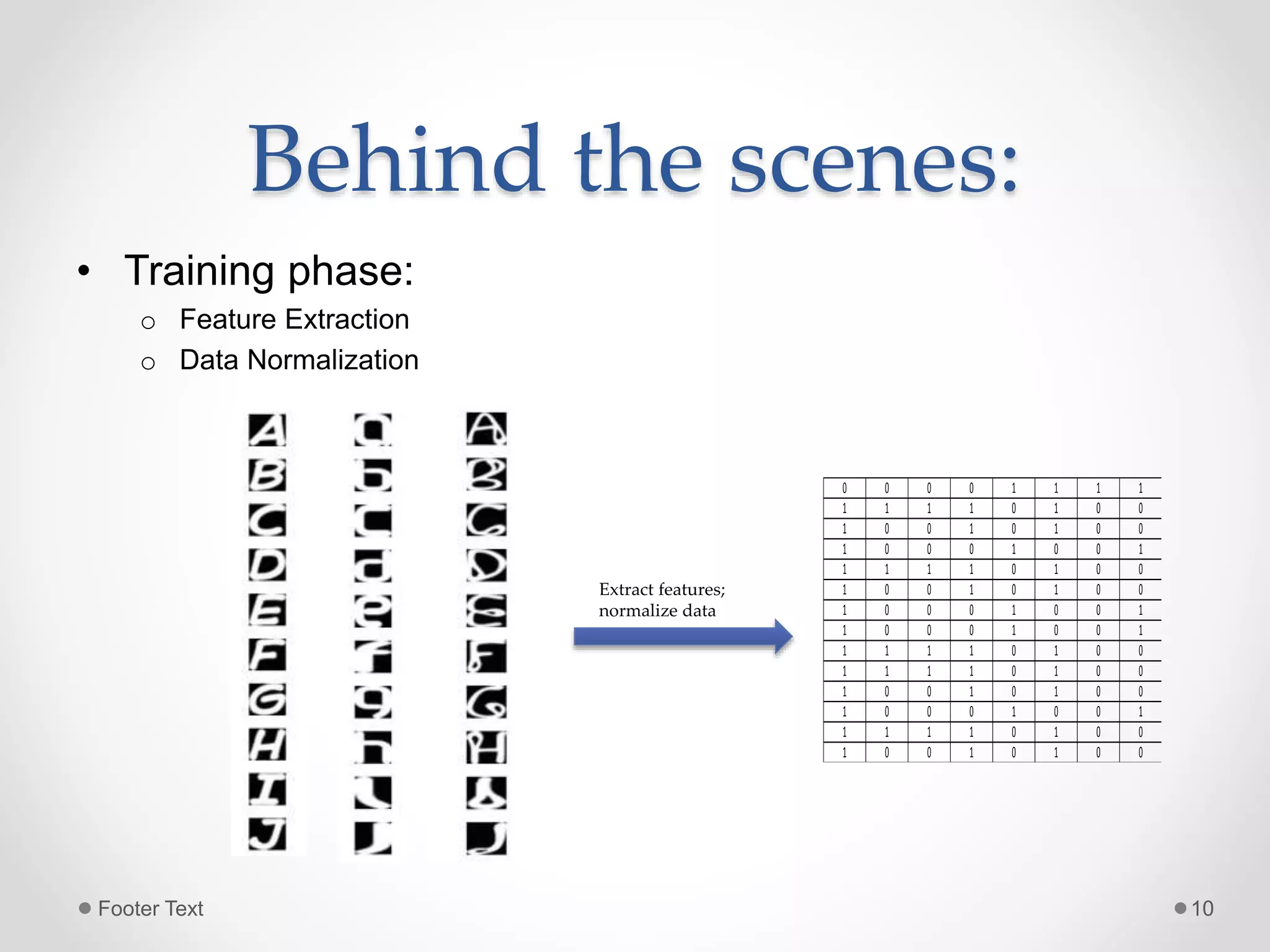
Behind the scenes: • Training phase: o Feature Extraction o Data Normalization Extract features; normalize data 0 0 0 0 1 1 1 1 1 1 1 1 0 1 0 0 1 0 0 1 0 1 0 0 1 0 0 0 1 0 0 1 1 1 1 1 0 1 0 0 1 0 0 1 0 1 0 0 1 0 0 0 1 0 0 1 1 0 0 0 1 0 0 1 1 1 1 1 0 1 0 0 1 1 1 1 0 1 0 0 1 0 0 1 0 1 0 0 1 0 0 0 1 0 0 1 1 1 1 1 0 1 0 0 1 0 0 1 0 1 0 0 Footer Text 10

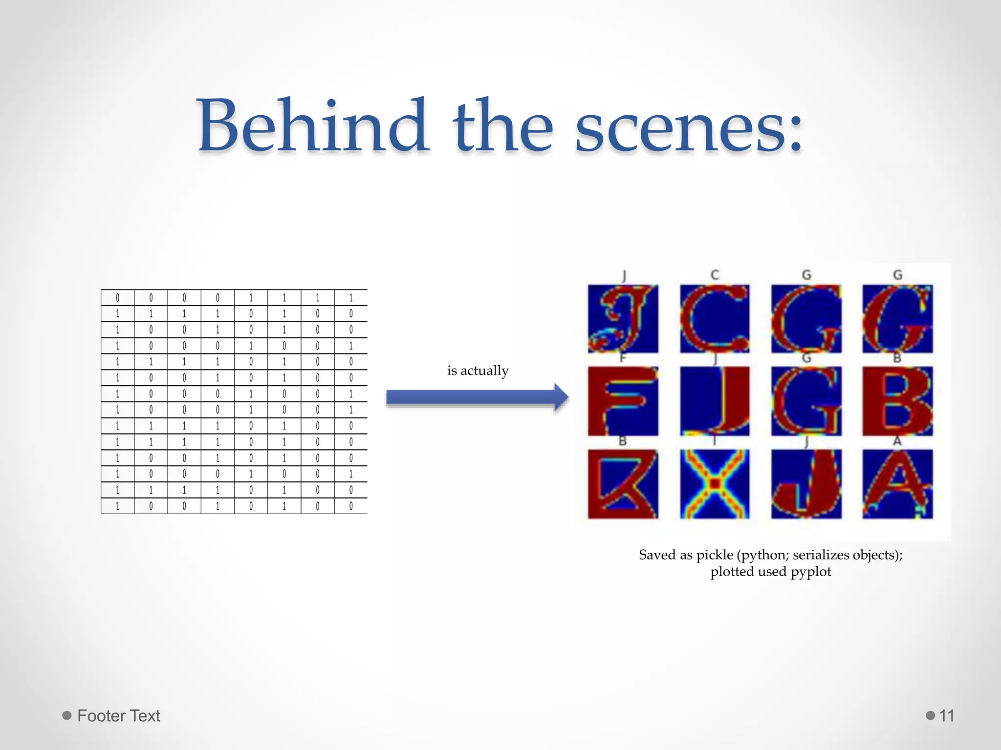
Behind the scenes: is actually 0 0 0 0 1 1 1 1 1 1 1 1 0 1 0 0 1 0 0 1 0 1 0 0 1 0 0 0 1 0 0 1 1 1 1 1 0 1 0 0 1 0 0 1 0 1 0 0 1 0 0 0 1 0 0 1 1 0 0 0 1 0 0 1 1 1 1 1 0 1 0 0 1 1 1 1 0 1 0 0 1 0 0 1 0 1 0 0 1 0 0 0 1 0 0 1 1 1 1 1 0 1 0 0 1 0 0 1 0 1 0 0 Saved as pickle (python; serializes objects); plotted used pyplot Footer Text 11

Behind the scenes: • Training phase: o Model • Learn weights/ parameters based on training data o Goal: Minimize loss • Function: Logistic Regression (aka logit) o y = wTx + b • w: weights ; x: features ; b: bias terms used for regularization • y: predicted value • Minimize: gradient descent approach/ stochastic gradient descent o Iterative process Footer Text 12

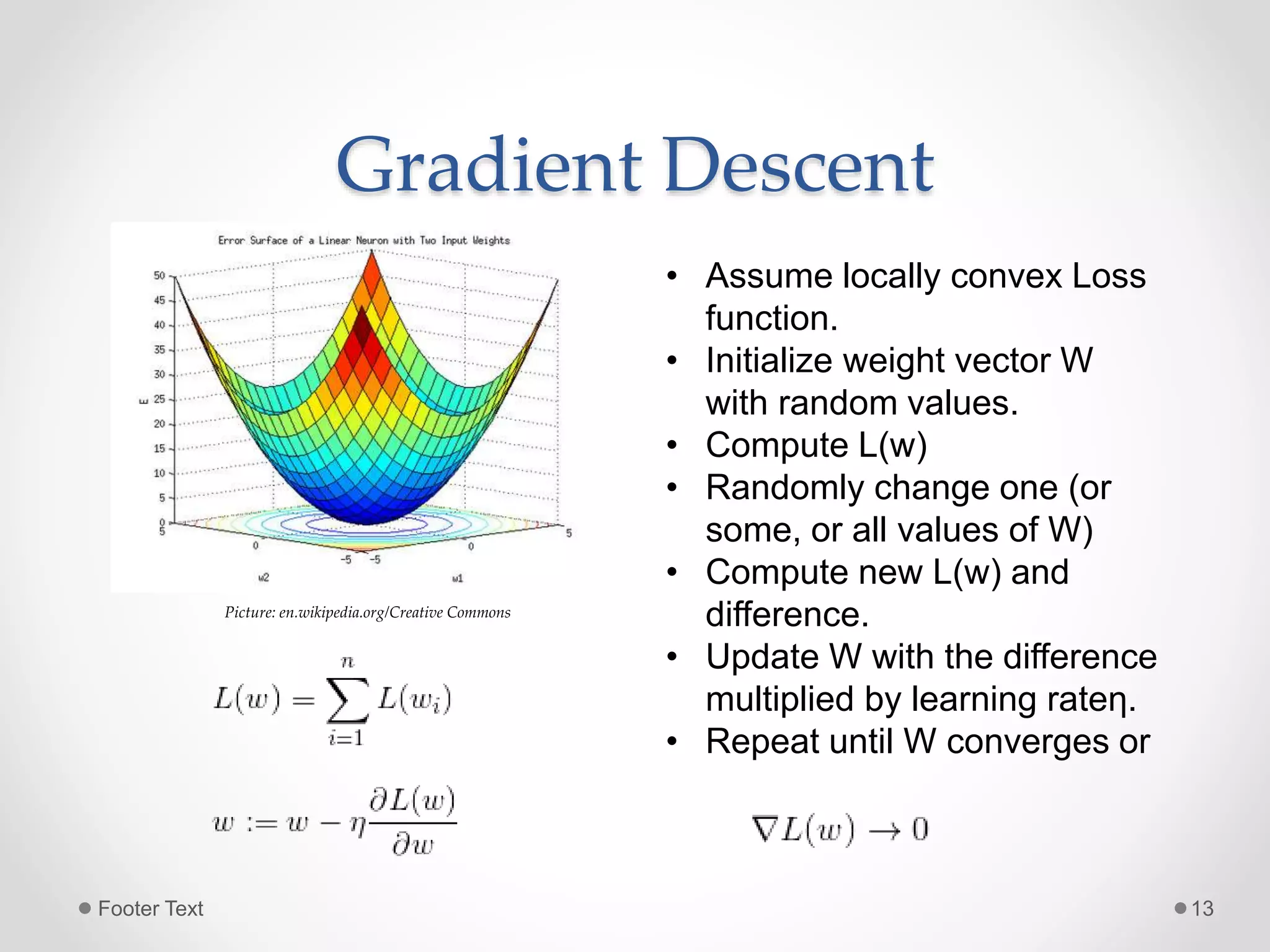
Gradient Descent Picture: en.wikipedia.org/Creative Commons • Assume locally convex Loss function. • Initialize weight vector W with random values. • Compute L(w) • Randomly change one (or some, or all values of W) • Compute new L(w) and difference. • Update W with the difference multiplied by learning rateη. • Repeat until W converges or Footer Text 13

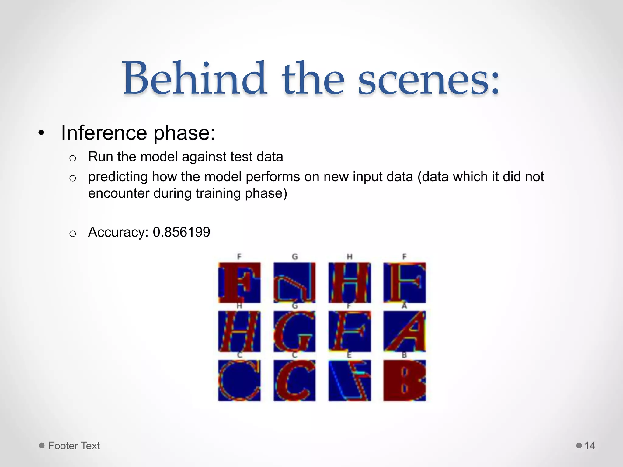
Behind the scenes: • Inference phase: o Run the model against test data o predicting how the model performs on new input data (data which it did not encounter during training phase) o Accuracy: 0.856199 Footer Text 14

Another example • Classify email as spam or not o https://github.com/abhi21/Spam-Classifier-NB Footer Text 15

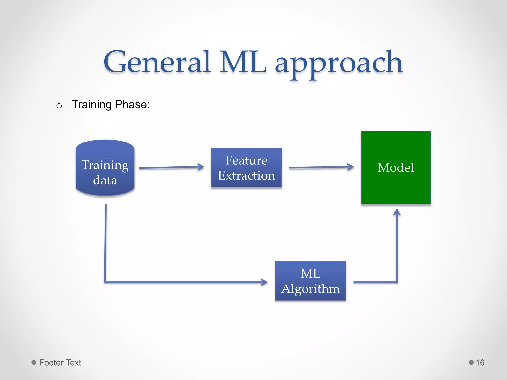
General ML approach o Training Phase: Training data Feature Extraction Model ML Algorithm Footer Text 16

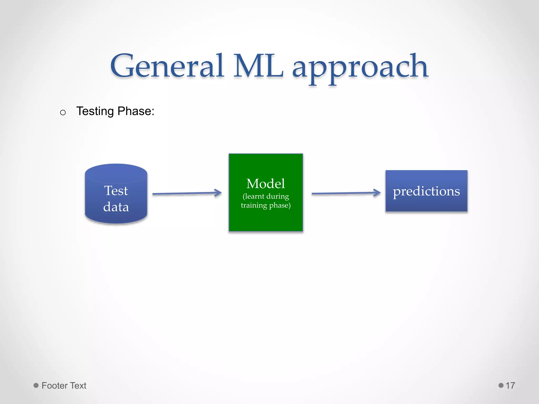
General ML approach o Testing Phase: Test data Model (learnt during training phase) predictions Footer Text 17

Need for Deep Learning • Pros • Automatic Feature Selection. • Ability to re-use basic building blocks to compose models tailored to different applications. • Cons • Tendency to over fit. • Requires lots of data. Footer Text 18

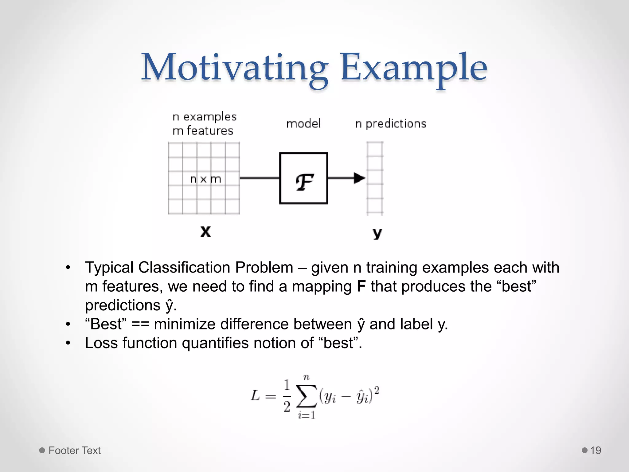
Motivating Example • Typical Classification Problem – given n training examples each with m features, we need to find a mapping F that produces the “best” predictions ŷ. • “Best” == minimize difference between ŷ and label y. • Loss function quantifies notion of “best”. Footer Text 19

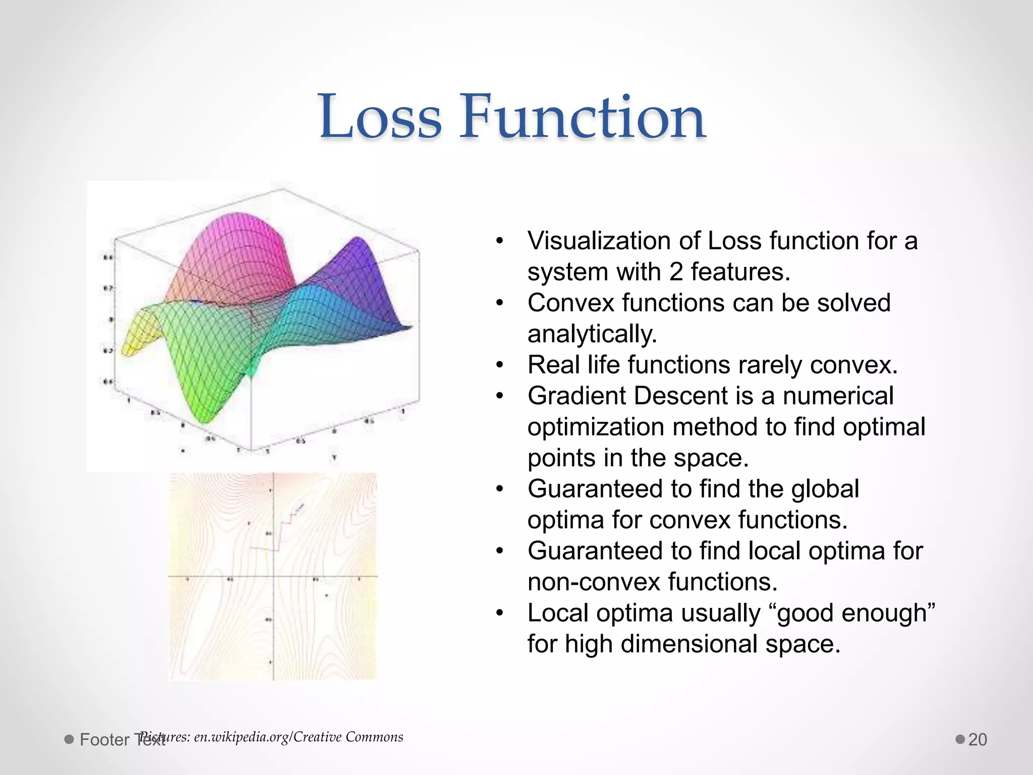
Loss Function • Visualization of Loss function for a system with 2 features. • Convex functions can be solved analytically. • Real life functions rarely convex. • Gradient Descent is a numerical optimization method to find optimal points in the space. • Guaranteed to find the global optima for convex functions. • Guaranteed to find local optima for non-convex functions. • Local optima usually “good enough” for high dimensional space. Pictures: en.wikipedia.org/Creative CommonsFooter Text 20

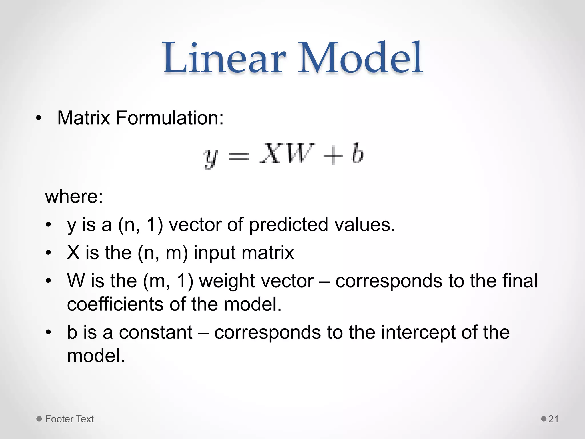
Linear Model • Matrix Formulation: where: • y is a (n, 1) vector of predicted values. • X is the (n, m) input matrix • W is the (m, 1) weight vector – corresponds to the final coefficients of the model. • b is a constant – corresponds to the intercept of the model. Footer Text 21

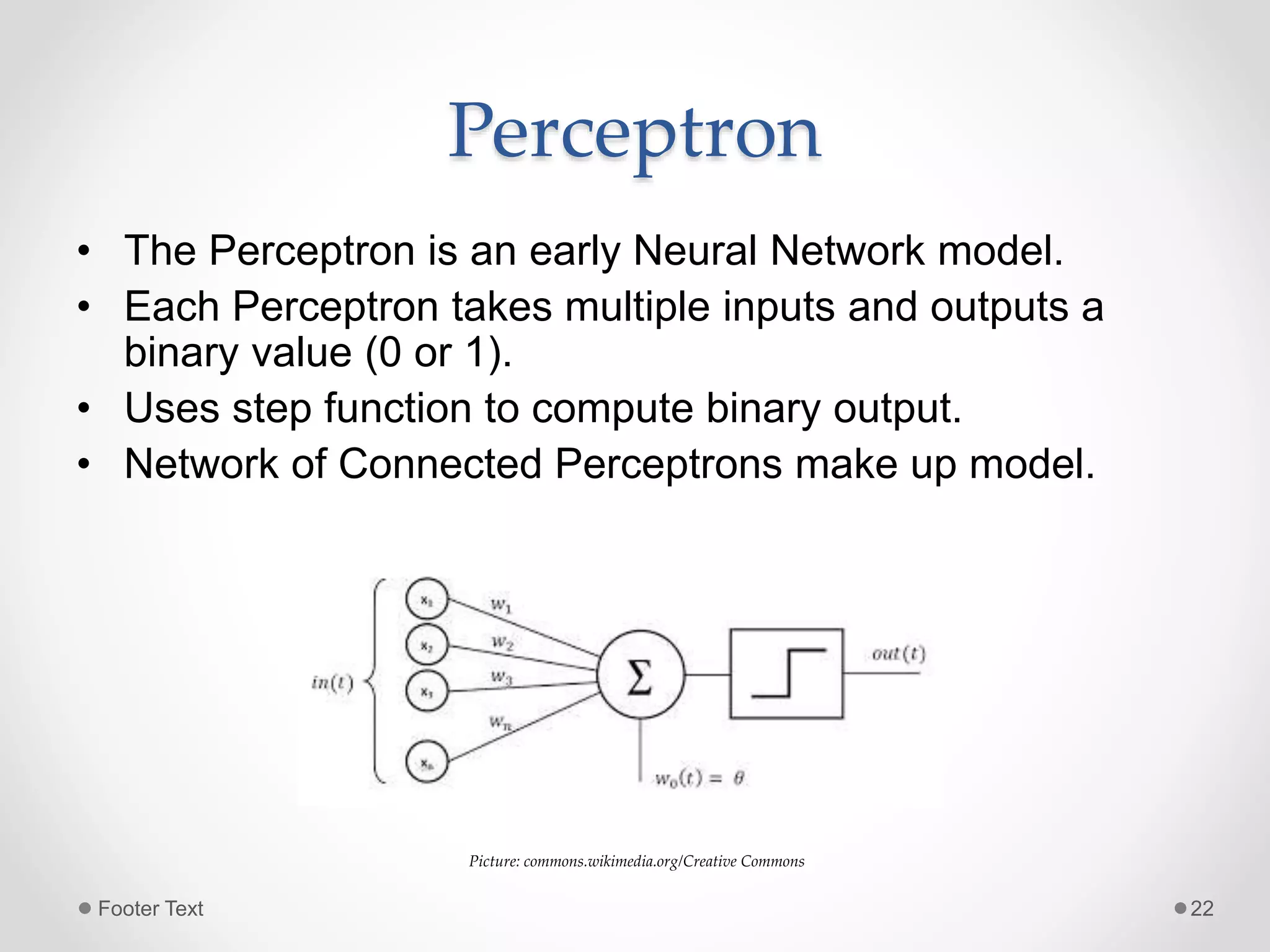
Perceptron • The Perceptron is an early Neural Network model. • Each Perceptron takes multiple inputs and outputs a binary value (0 or 1). • Uses step function to compute binary output. • Network of Connected Perceptrons make up model. Picture: commons.wikimedia.org/Creative Commons Footer Text 22

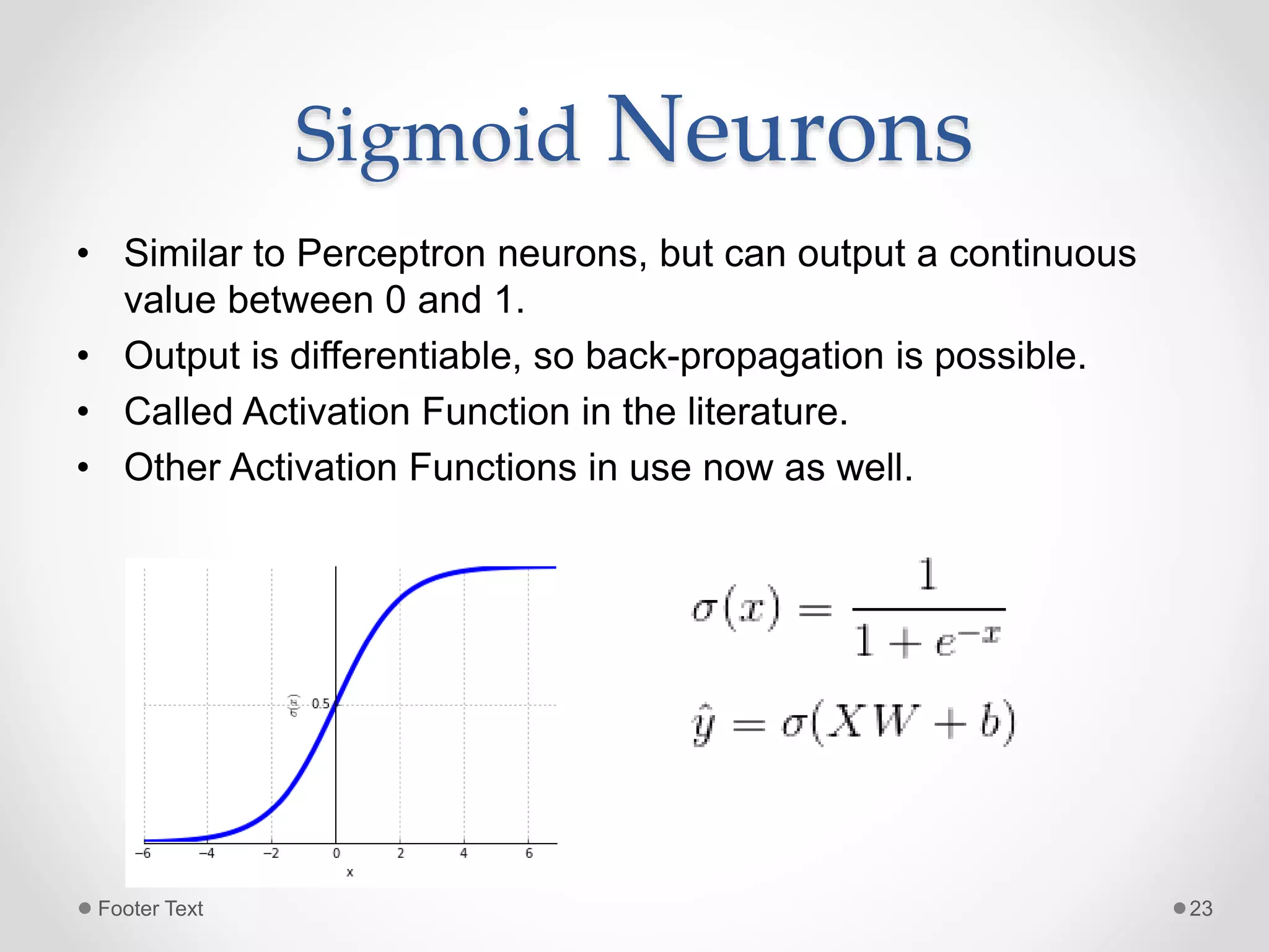
Sigmoid Neurons • Similar to Perceptron neurons, but can output a continuous value between 0 and 1. • Output is differentiable, so back-propagation is possible. • Called Activation Function in the literature. • Other Activation Functions in use now as well. Footer Text 23

Popular Toolkits • Comprehensive List in the PyImageSearch blog My Top 9 Favorite Python Deep Learning Libraries from Adrian Rosenbrock. • I use the following. o Caffe – written in C++, network architectures defined using JSON, has Python interface for training and running networks. Very mature and has many prebuilt models. o Keras – Python wrapper that exposes very minimal and easy to use interface. Useful if you are composing your architectures from existing models. o Tensorflow – written in C++ but Python API gives you full control over the network. Useful if you are building new architectures (or those not available already) Footer Text 24

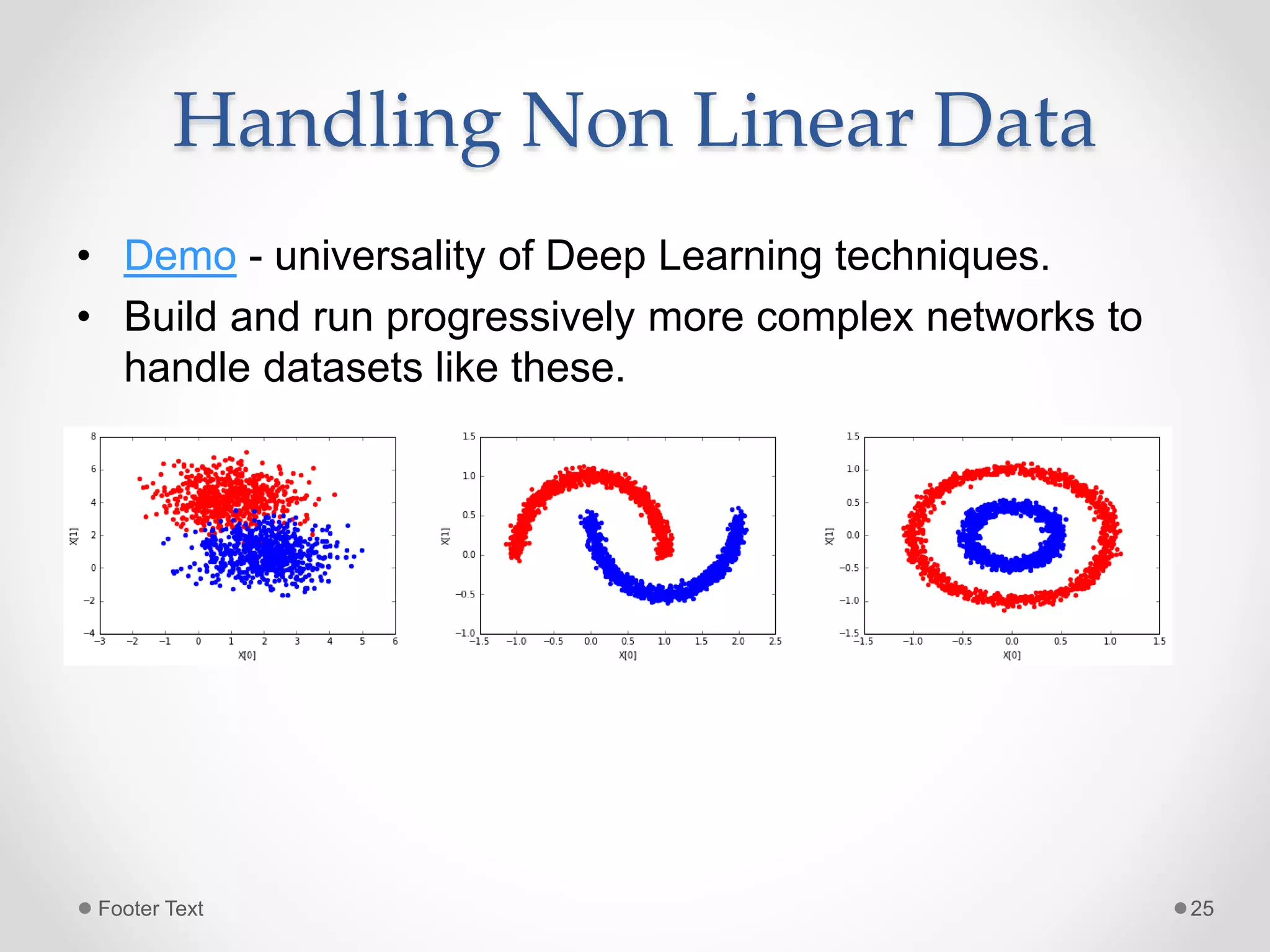
Handling Non Linear Data • Demo - universality of Deep Learning techniques. • Build and run progressively more complex networks to handle datasets like these. Footer Text 25

Building Blocks • Fully Connected Networks o First network model to become popular in Deep Learning. o Has been applied to classification, generating embeddings for natural language vocabularies, etc. • Convolutional Neural Networks o Exploits the geometry of the input. o Applied to computer vision (image and video), classification and natural language processing. • Recurrent Neural Networks o Exploits the temporal nature of the input. o Applied to classification, audio and speech applications, natural language processing, machine translation, image captioning, etc. Footer Text 26

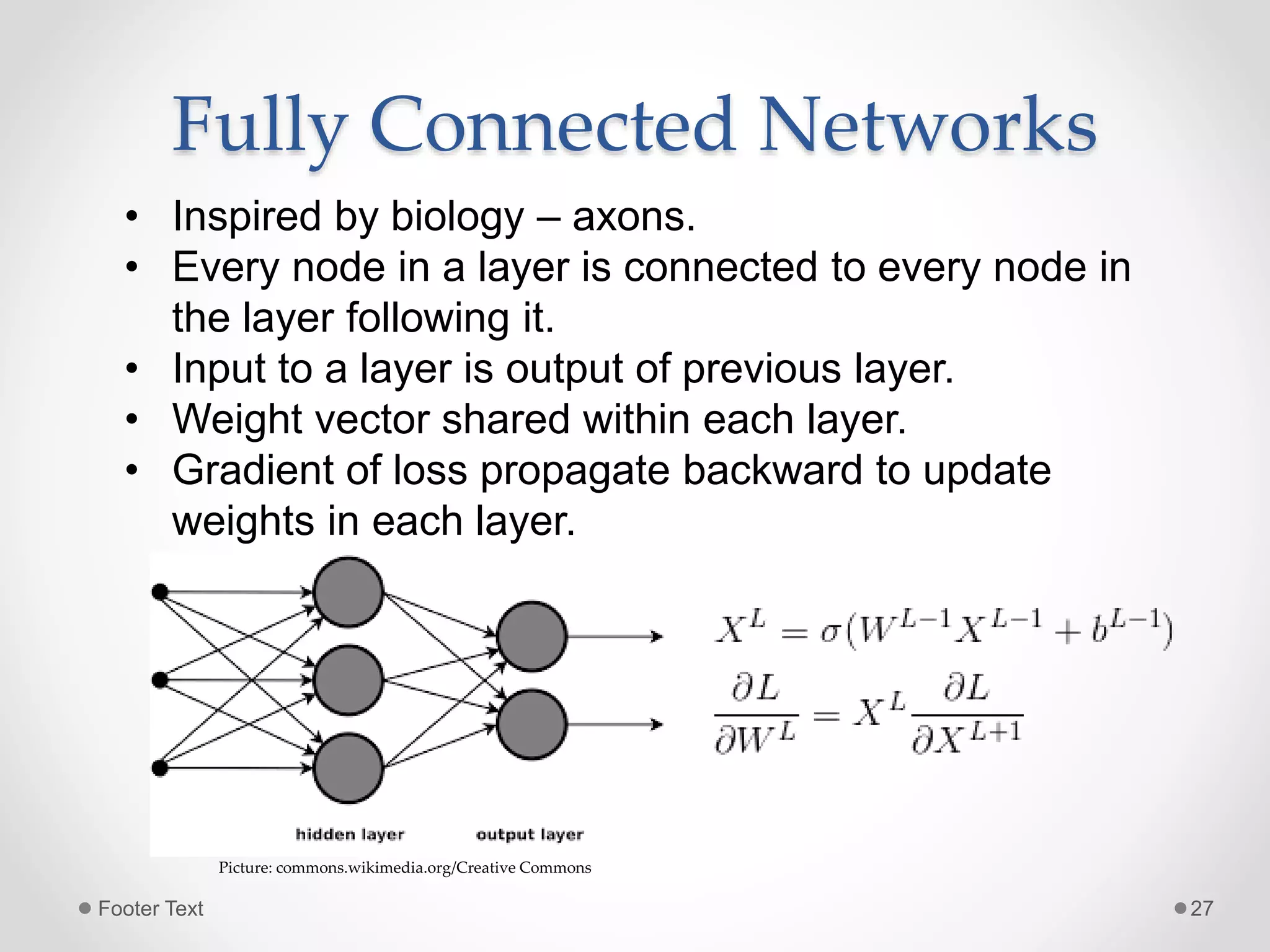
Fully Connected Networks • Inspired by biology – axons. • Every node in a layer is connected to every node in the layer following it. • Input to a layer is output of previous layer. • Weight vector shared within each layer. • Gradient of loss propagate backward to update weights in each layer. Picture: commons.wikimedia.org/Creative Commons Footer Text 27

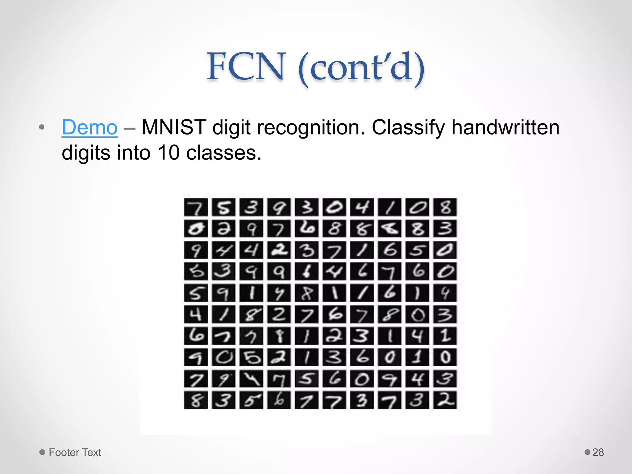
FCN (cont’d) • Demo – MNIST digit recognition. Classify handwritten digits into 10 classes. Footer Text 28

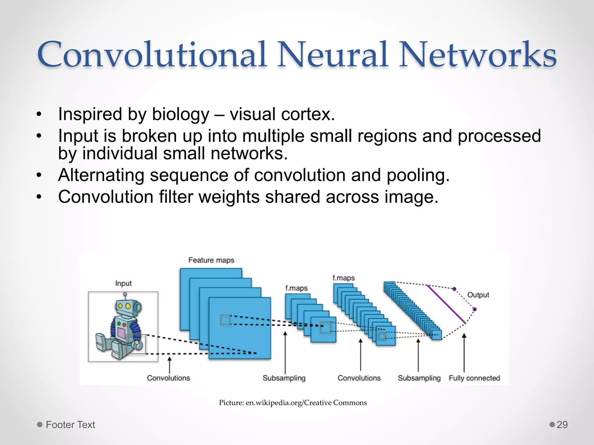
Convolutional Neural Networks • Inspired by biology – visual cortex. • Input is broken up into multiple small regions and processed by individual small networks. • Alternating sequence of convolution and pooling. • Convolution filter weights shared across image. Picture: en.wikipedia.org/Creative Commons Footer Text 29

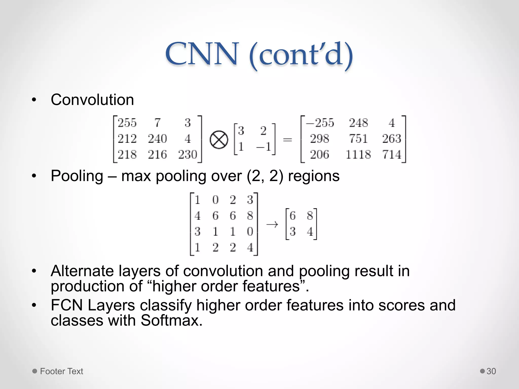
CNN (cont’d) • Convolution • Pooling – max pooling over (2, 2) regions • Alternate layers of convolution and pooling result in production of “higher order features”. • FCN Layers classify higher order features into scores and classes with Softmax. Footer Text 30

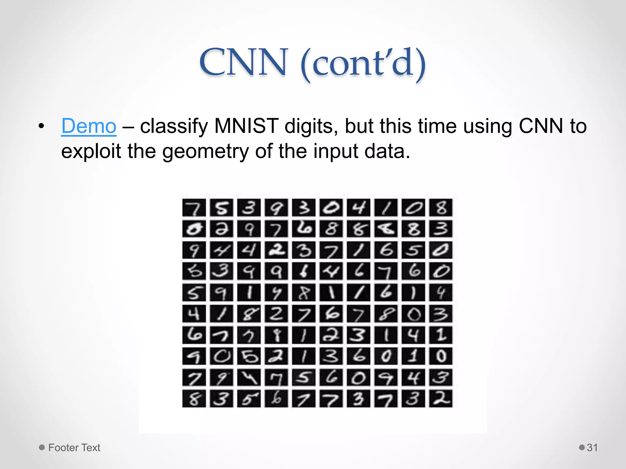
CNN (cont’d) • Demo – classify MNIST digits, but this time using CNN to exploit the geometry of the input data. Footer Text 31

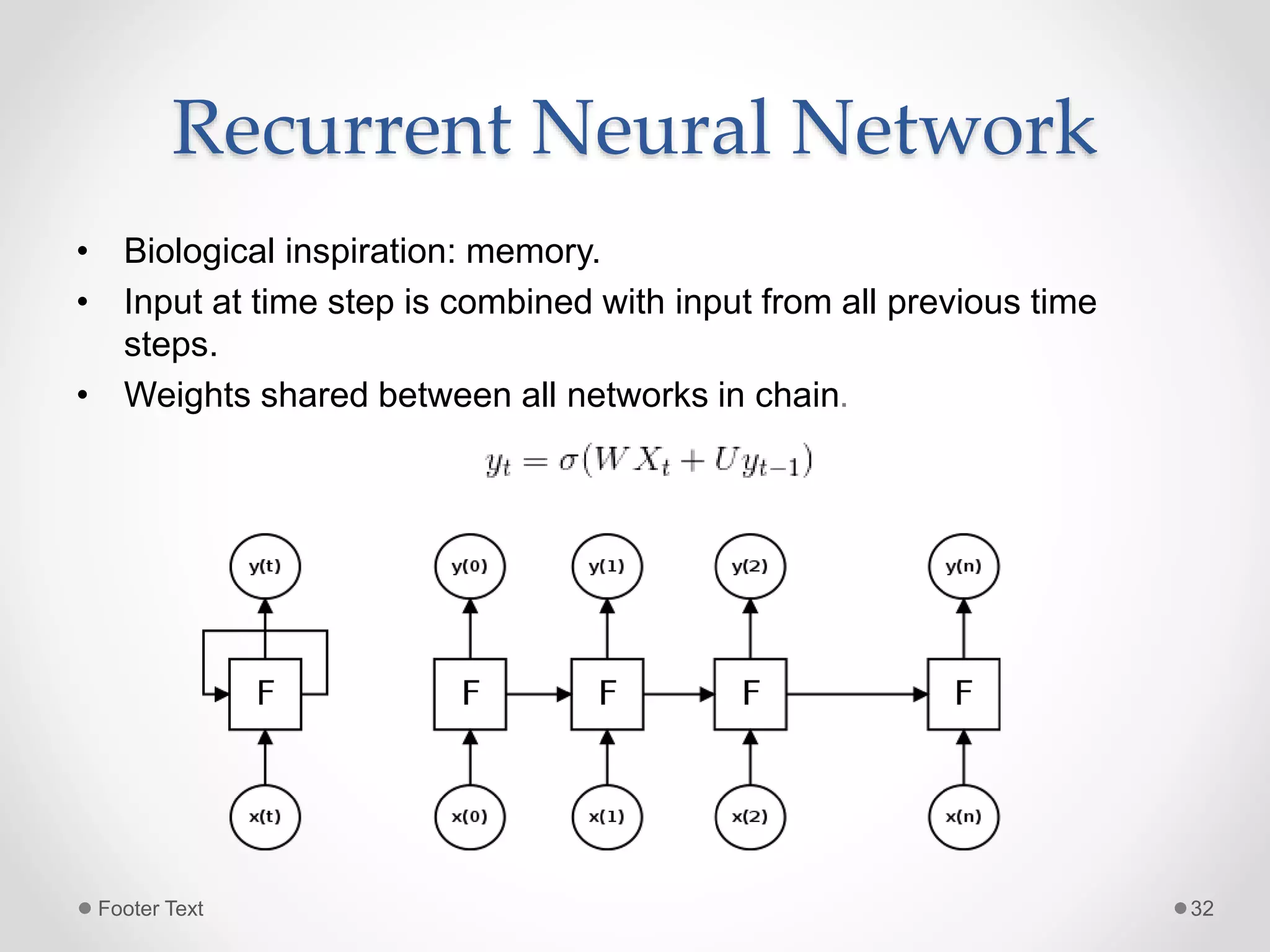
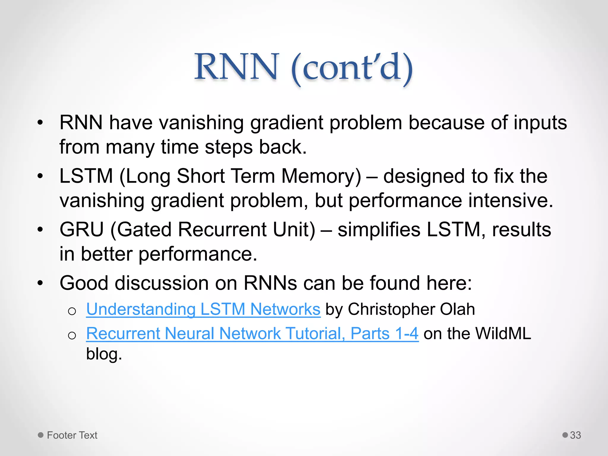
Recurrent Neural Network • Biological inspiration: memory. • Input at time step is combined with input from all previous time steps. • Weights shared between all networks in chain. Footer Text 32

RNN (cont’d) • RNN have vanishing gradient problem because of inputs from many time steps back. • LSTM (Long Short Term Memory) – designed to fix the vanishing gradient problem, but performance intensive. • GRU (Gated Recurrent Unit) – simplifies LSTM, results in better performance. • Good discussion on RNNs can be found here: o Understanding LSTM Networks by Christopher Olah o Recurrent Neural Network Tutorial, Parts 1-4 on the WildML blog. Footer Text 33

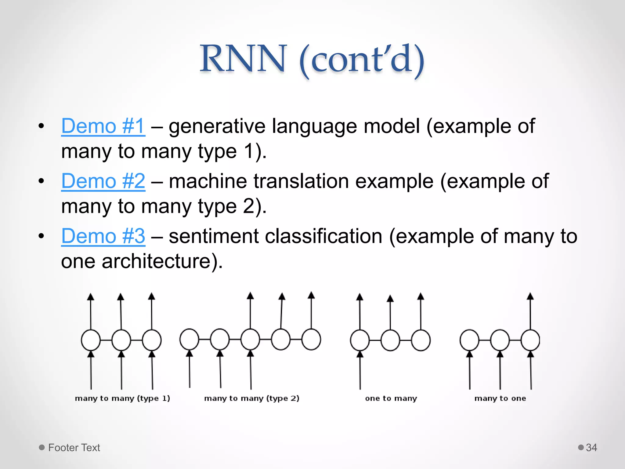
RNN (cont’d) • Demo #1 – generative language model (example of many to many type 1). • Demo #2 – machine translation example (example of many to many type 2). • Demo #3 – sentiment classification (example of many to one architecture). Footer Text 34

Conclusion Artificial Intelligence Machine Learning Deep Learning Footer Text 35

Learn More! Note: many concepts were not covered! • Machine Learning (Tom M. Mitchell) • Pattern Recognition and Machine Learning (Christopher Bishop) • MOOCs: o Machine Learning – covers almost all the important concepts in Machine Learning o Deep Learning on Udacity – good coverage of the basics of Deep Learning and Tensorflow. o CS224d on Stanford – Deep Learning for Natural Language Processing, taught by Richard Socher. o CS231n on Stanford – Convolutional Neural Networks for Visual Recognition. • Deep Learning Enthusiasts meetup group Footer Text 36

References • Google Trends • notMNIST Dataset: http://yaroslavvb.blogspot.com/2011/09/notmnist-dataset.html • http://www.cs.princeton.edu/courses/archive/spr08/cos511/scribe_no tes/0204.pdf • https://classroom.udacity.com/courses/ud730/ Footer Text 37

Artificial Intelligence, Machine Learning and Deep Learning

More Related Content

What's hot

Viewers also liked

Similar to Artificial Intelligence, Machine Learning and Deep Learning

More from Sujit Pal

Recently uploaded

In this document

Artificial Intelligence, Machine Learning and Deep Learning