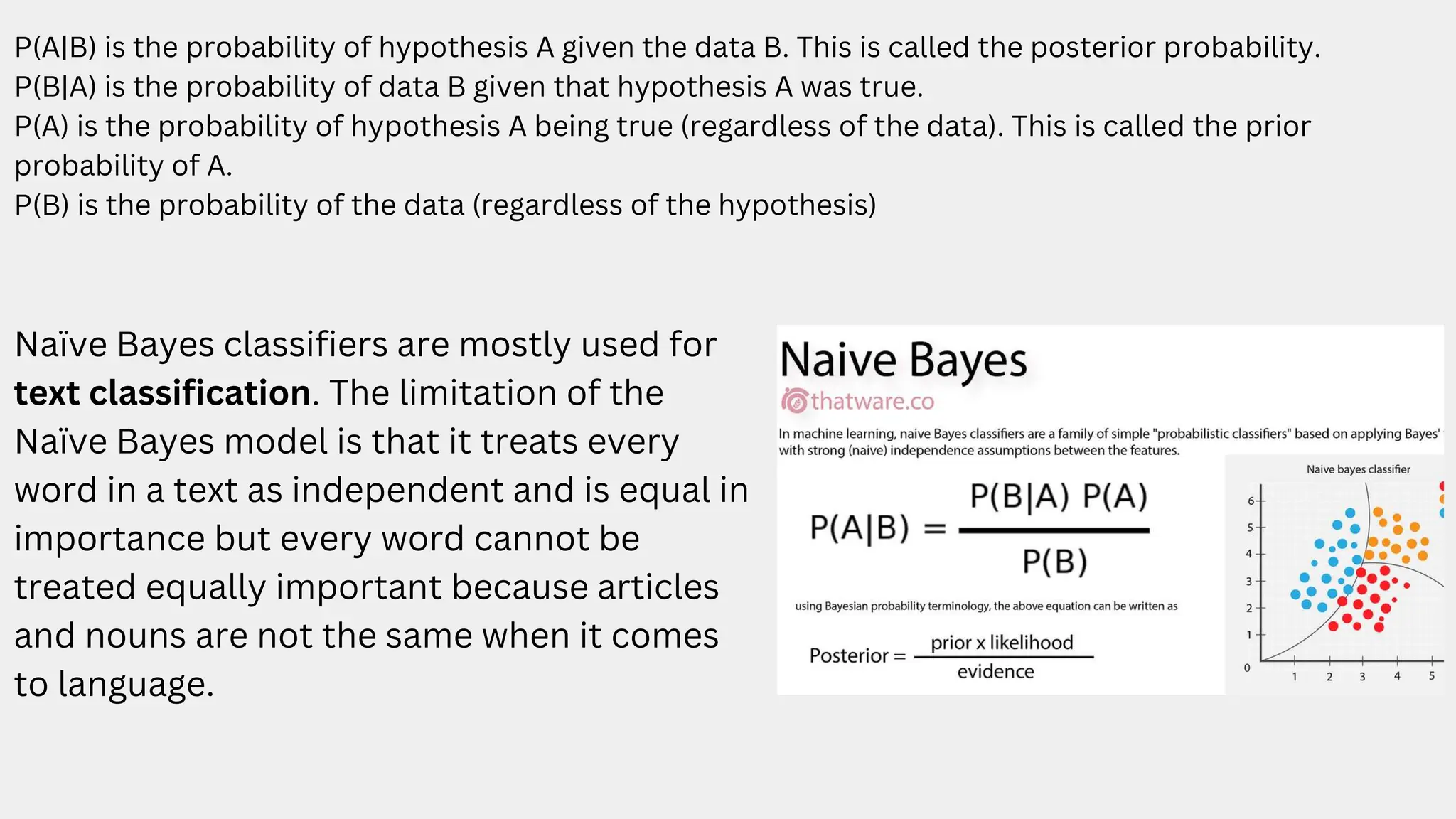
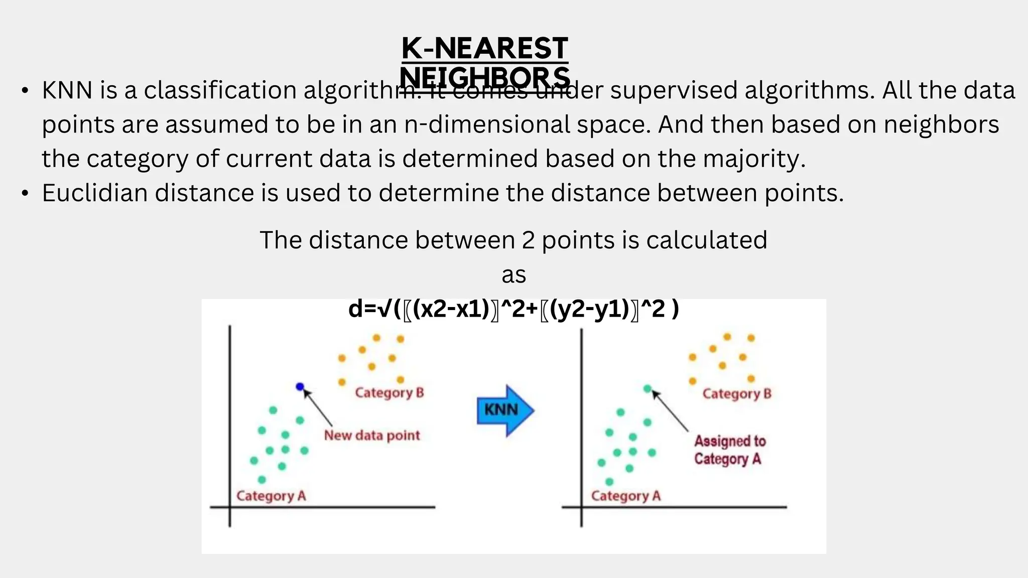
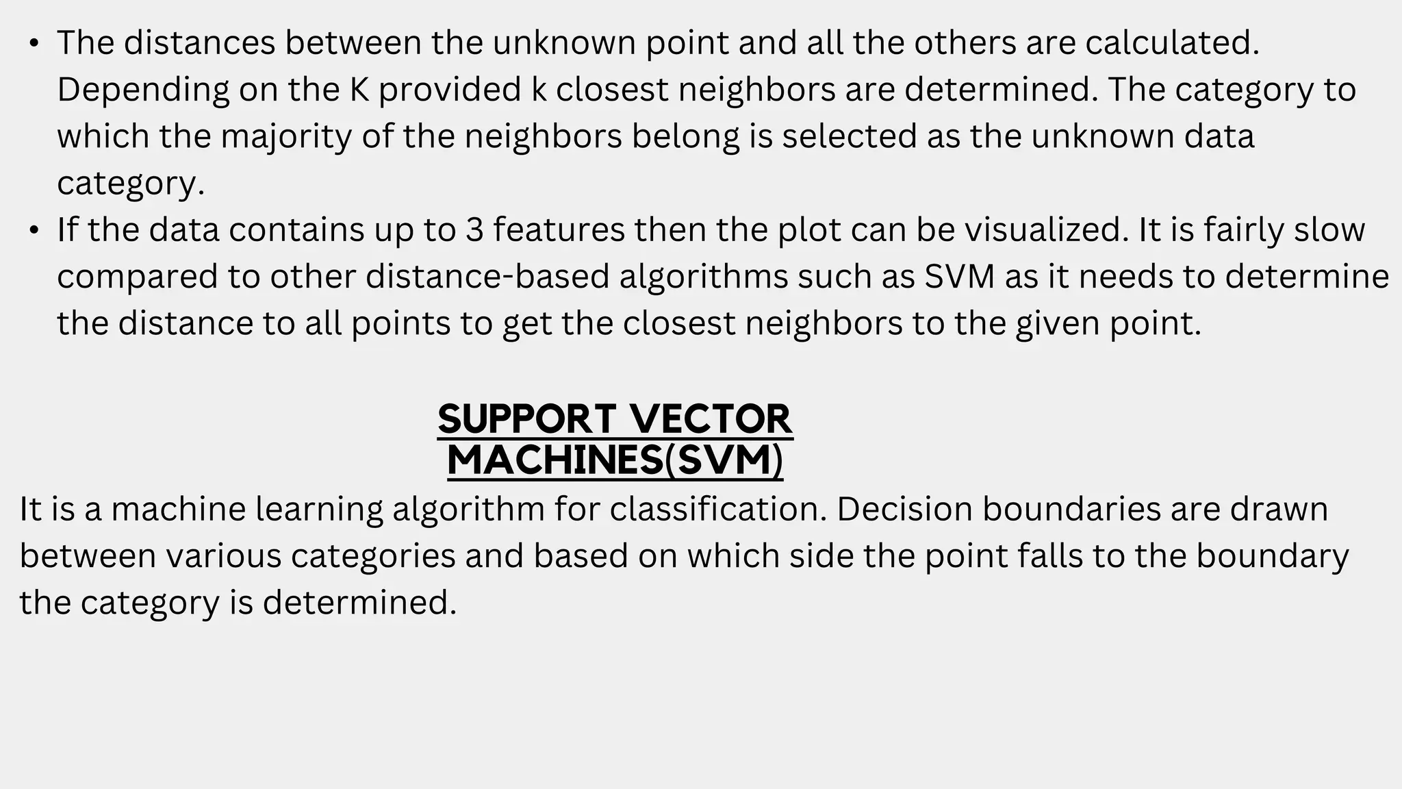
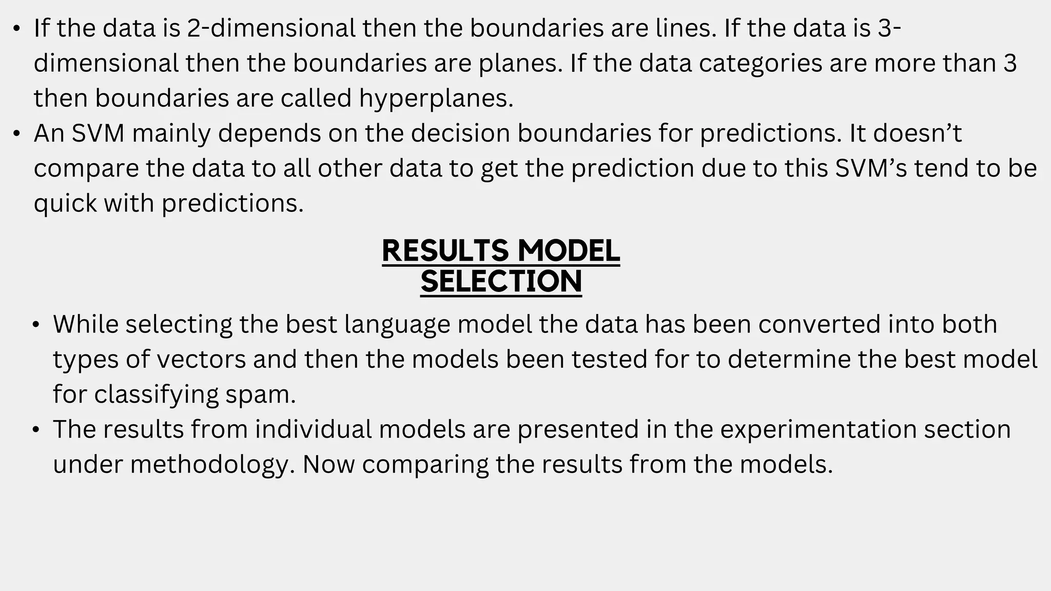
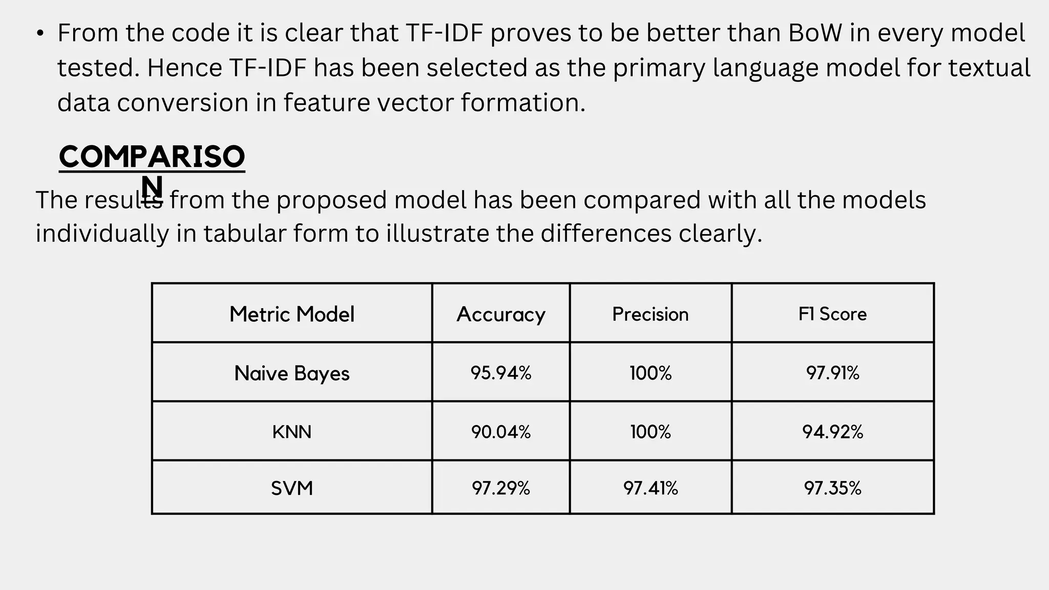
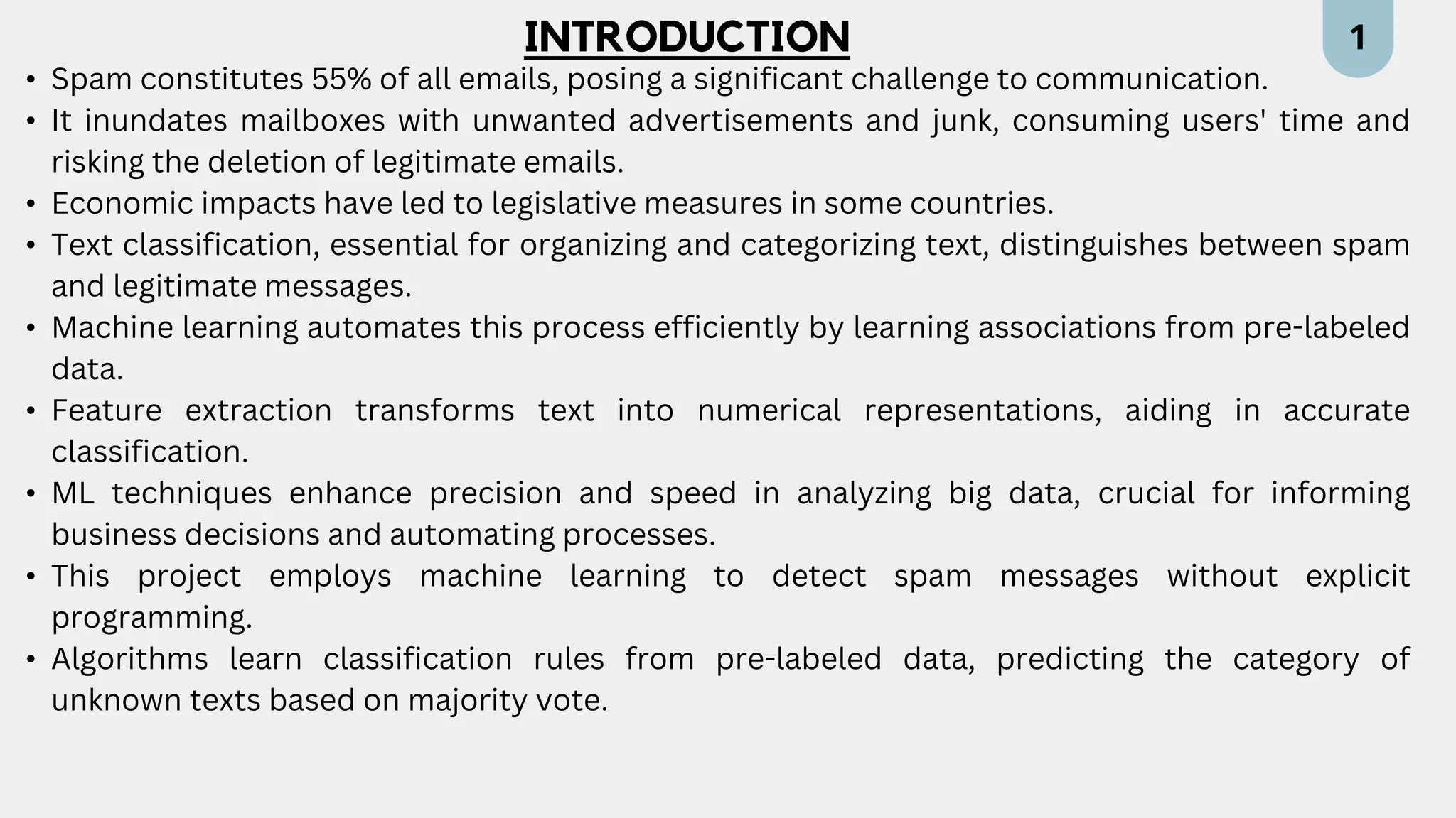
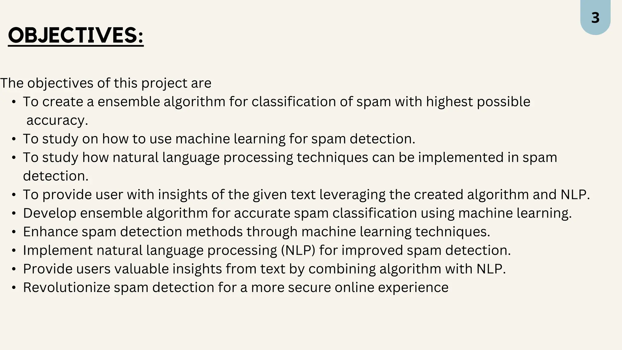
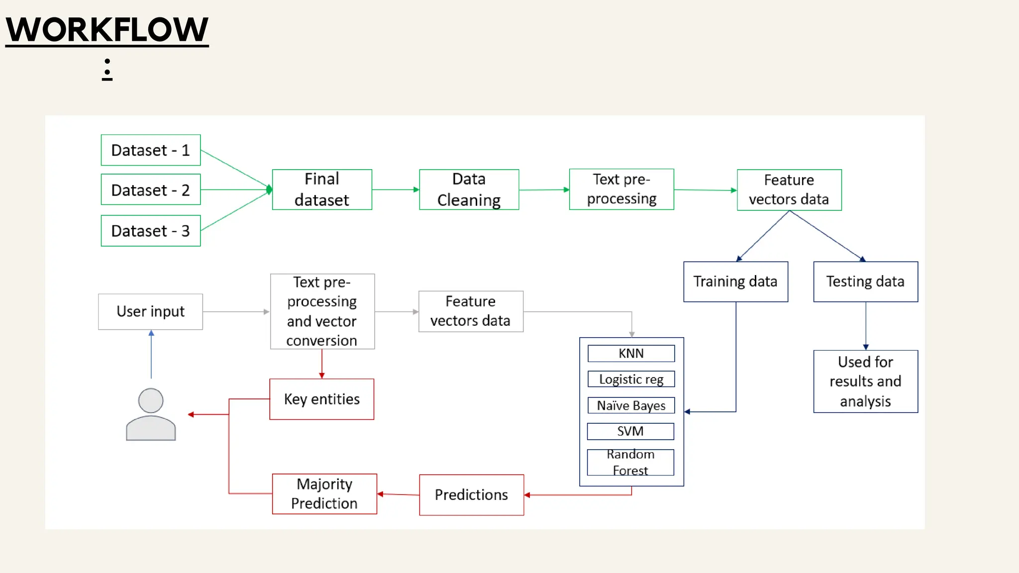
This document discusses a project aimed at developing an ensemble machine learning model for spam detection in emails, addressing the challenges posed by spammers and the need for effective filtering strategies. It highlights the use of natural language processing and various machine learning techniques, including naive bayes, k-nearest neighbors, and support vector machines, to improve classification accuracy. The results indicate that the term frequency-inverse document frequency (tf-idf) model outperforms the bag of words model, leading to a more effective spam detection system.

![BAG OF WORDS: Bag of words is a language model used mainly in text classification. A bag of words represents the text in a numerical form. The two things required for Bag of Words are • A vocabulary of words known to us. • A way to measure the presence of words. Ex: a few lines from the book “A Tale of Two Cities” by Charles Dickens. “ It was the best of times, it was the worst of times, it was the age of wisdom, it was the age of foolishness, ” The unique words here (ignoring case and punctuation) are: [ “it”, “was”, “the”, “best”, “of”, “times”, “worst”,“age”, “wisdom”, “foolishness” ] The next step is scoring words present in every document](https://image.slidesharecdn.com/datamining-240510151303-e93add0c/75/Data-Mining-Email-SPam-Detection-PPT-WITH-Algorithms-8-2048.jpg)
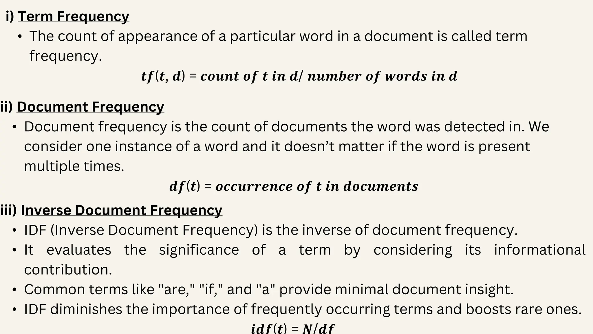
![After scoring the four lines from the above stanza can be represented in vector form as “It was the best of times“ = [1, 1, 1, 1, 1, 1, 0, 0, 0, 0] "it was the worst of times" = [1, 1, 1, 0, 1, 1, 1, 0, 0, 0] "it was the age of wisdom" = [1, 1, 1, 0, 1, 0, 0, 1, 1, 0] "it was the age of foolishness"= [1, 1, 1, 0, 1, 0, 0, 1, 0, 1] Term Frequency-Inverse Document Frequency: • Term frequency-inverse document frequency of a word is a measurement of the importance of a word. • It compares the repentance of words to the collection of documents and calculates the score. • Terminology for the below formulae: t – term(word). d – document. N – count of documents. The TF-IDF process consists of various activities listed below.](https://image.slidesharecdn.com/datamining-240510151303-e93add0c/75/Data-Mining-Email-SPam-Detection-PPT-WITH-Algorithms-9-2048.jpg)
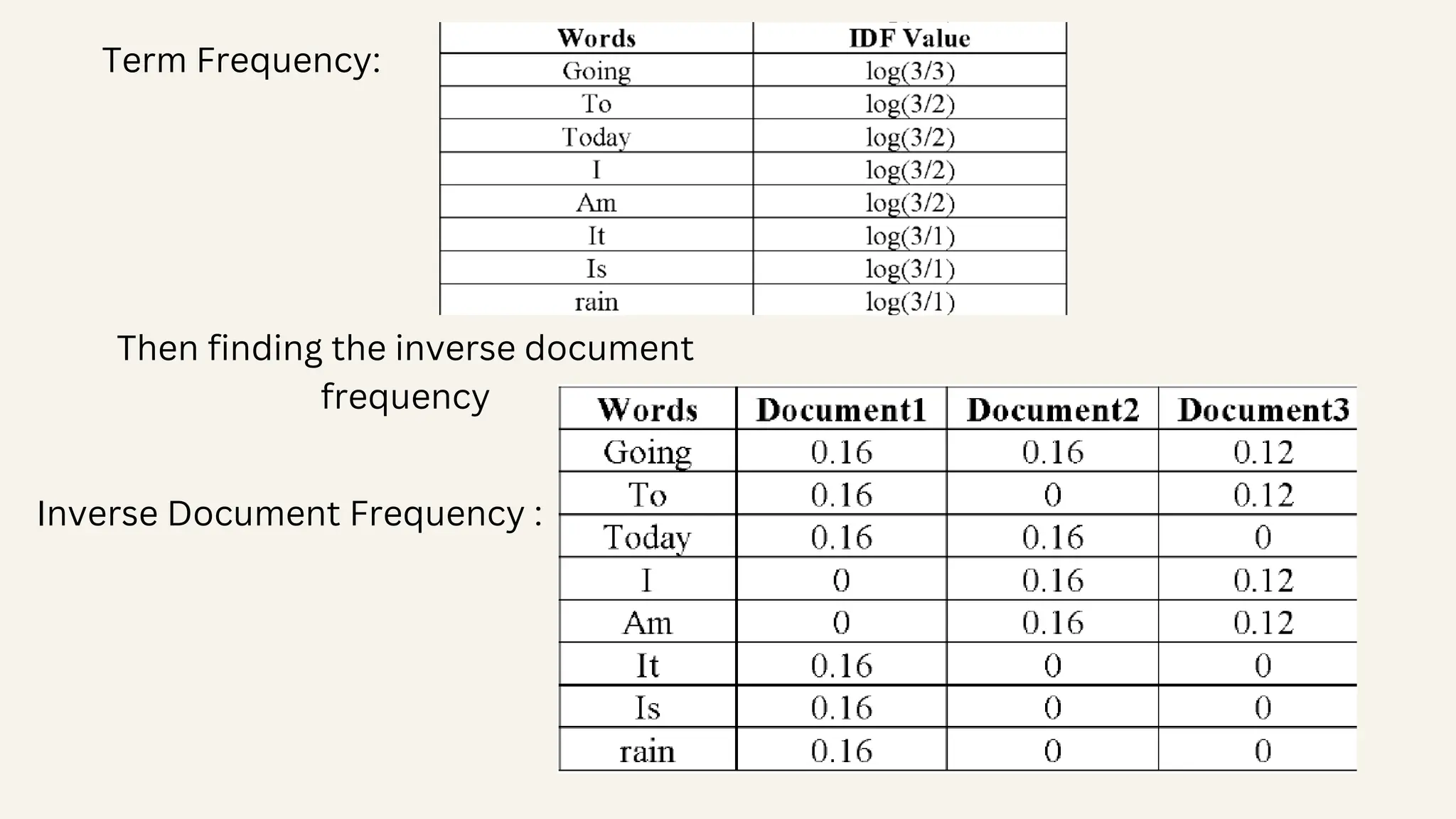
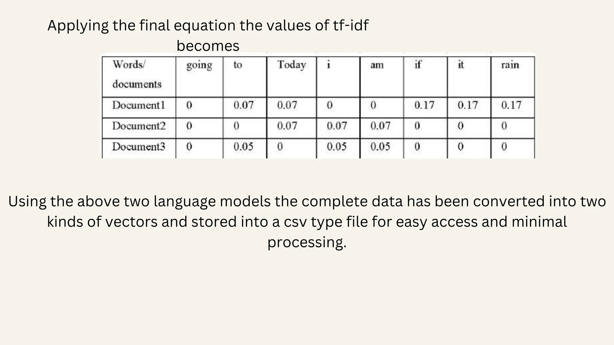
![Finally, the TF-IDF can be calculated by combining the term frequency and inverse document frequency. 𝒕𝒇_𝒊𝒅𝒇(𝒕, 𝒅) = 𝒕𝒇(𝒕, 𝒅) ∗ 𝐥𝐨 𝐠 (𝑵/(𝒅𝒇 + 𝟏)) The process can be explained using the following example: “Document 1 It is going to rain today. Document 2 Today I am not going outside. Document 3 I am going to watch the season premiere.” The Bag of words of the above sentences is [going:3, to:2, today:2, i:2, am:2, it:1, is:1, rain:1] • It combines term frequency (TF) and inverse document frequency (IDF). • TF represents the frequency of a word in a document, while IDF evaluates its significance across the collection. • By assigning weights to words, TF-IDF aids in text mining, information retrieval, and natural language processing.](https://image.slidesharecdn.com/datamining-240510151303-e93add0c/75/Data-Mining-Email-SPam-Detection-PPT-WITH-Algorithms-11-2048.jpg)