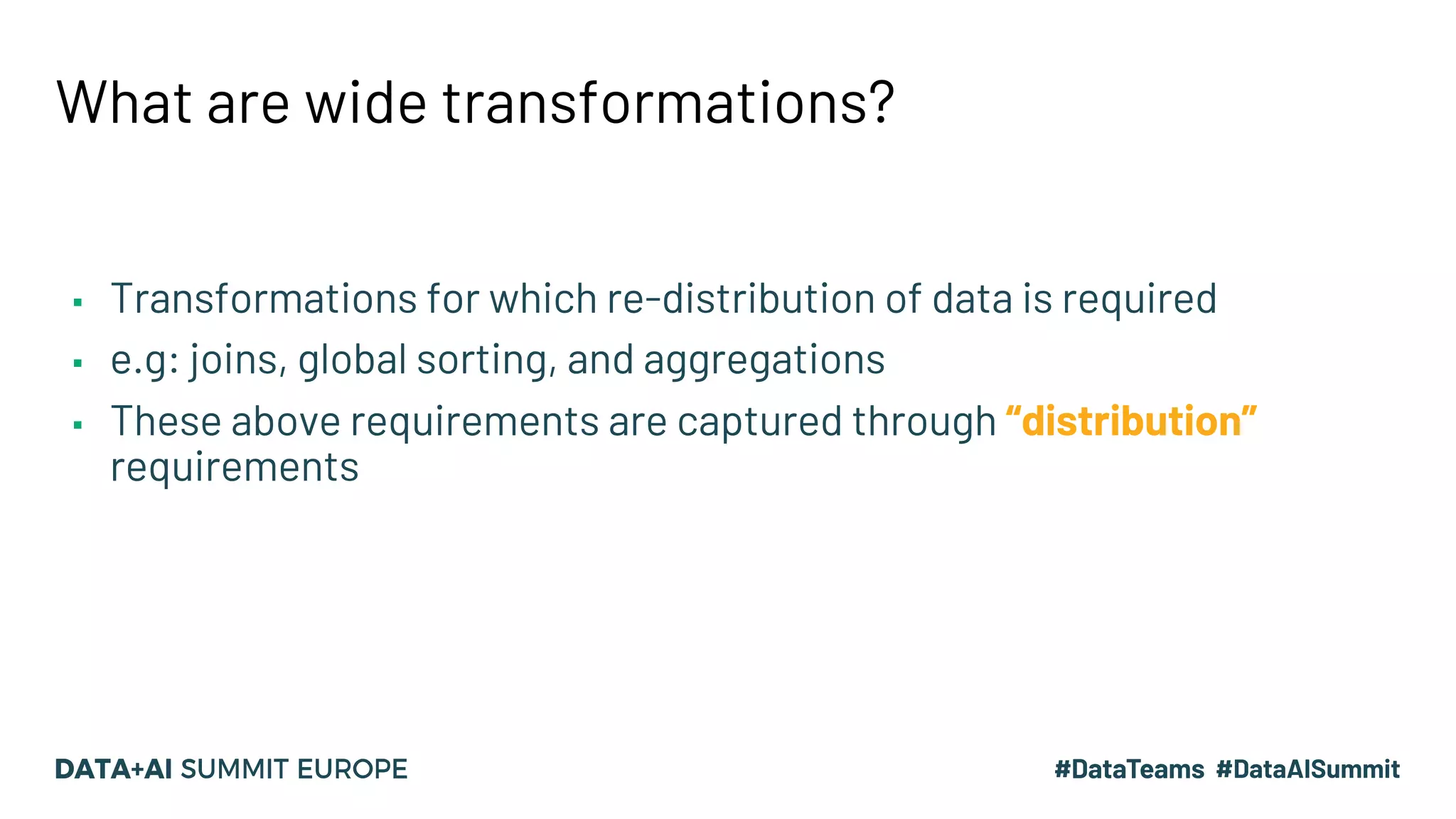
Download as PDF, PPTX


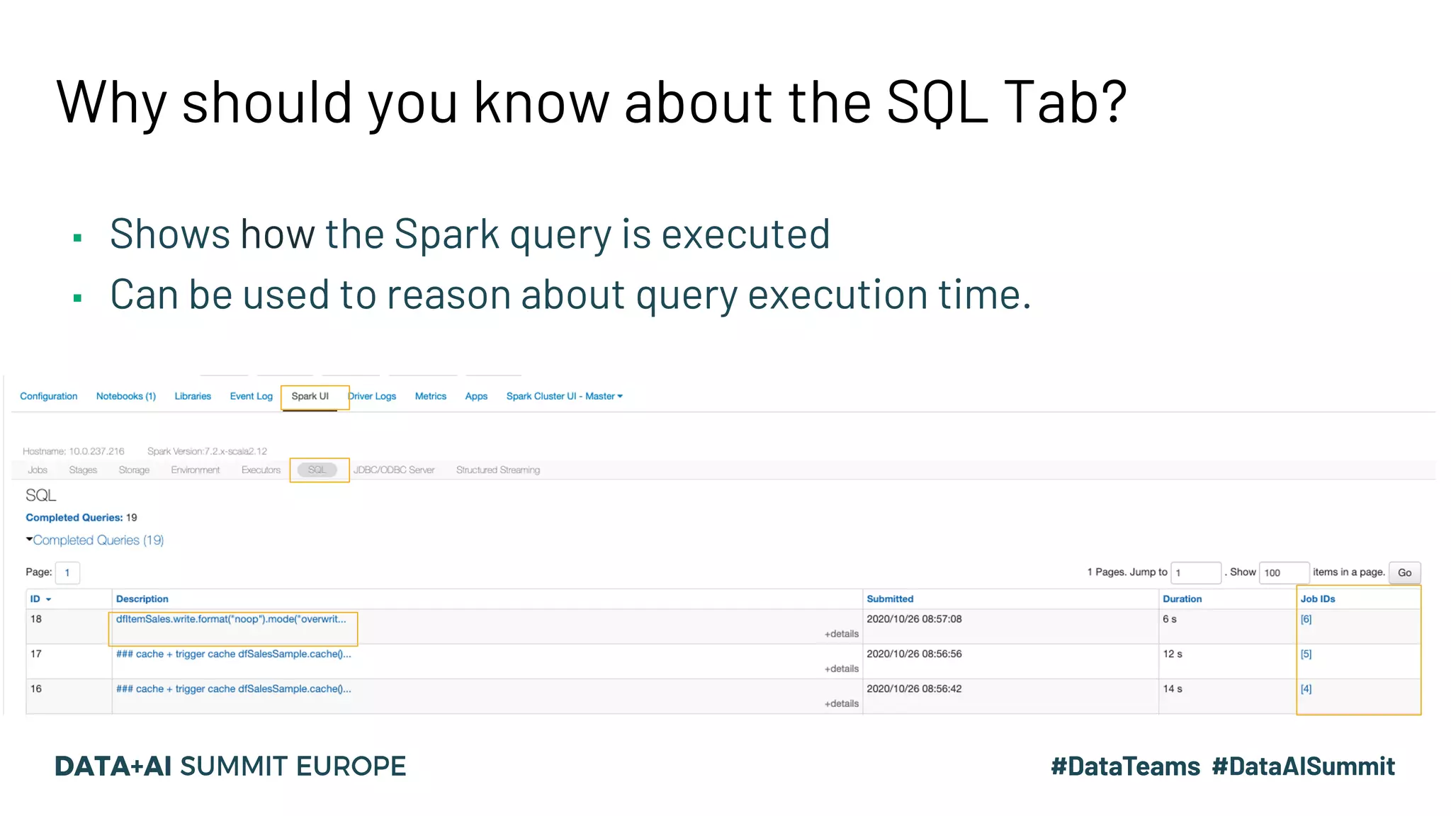
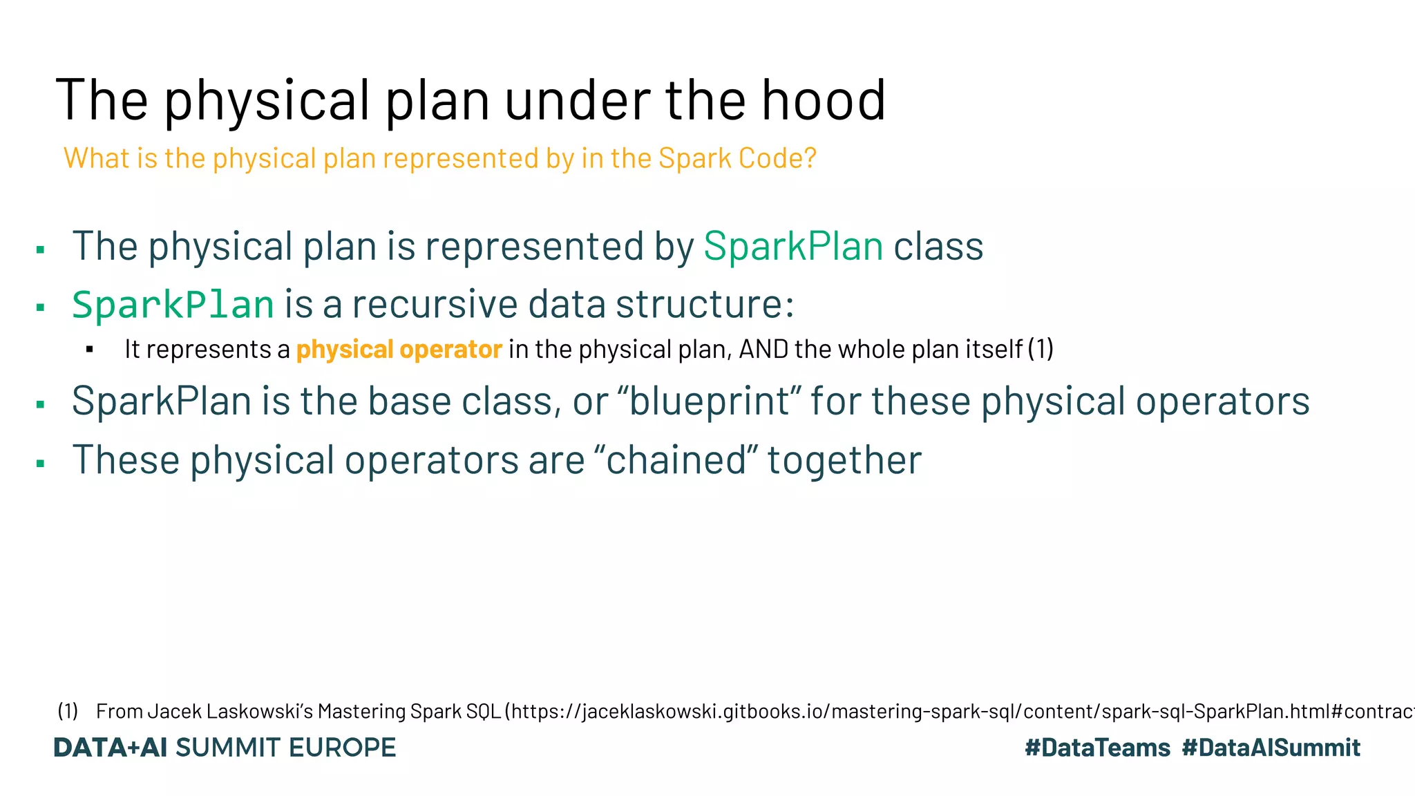
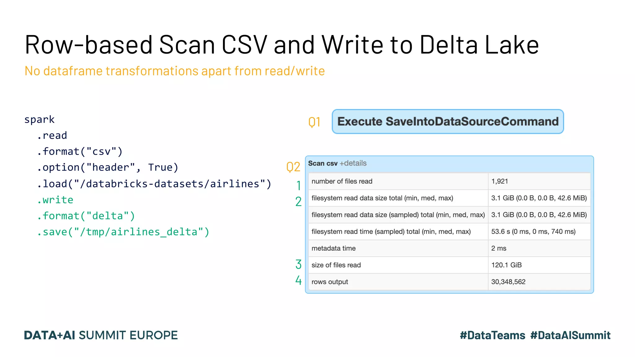
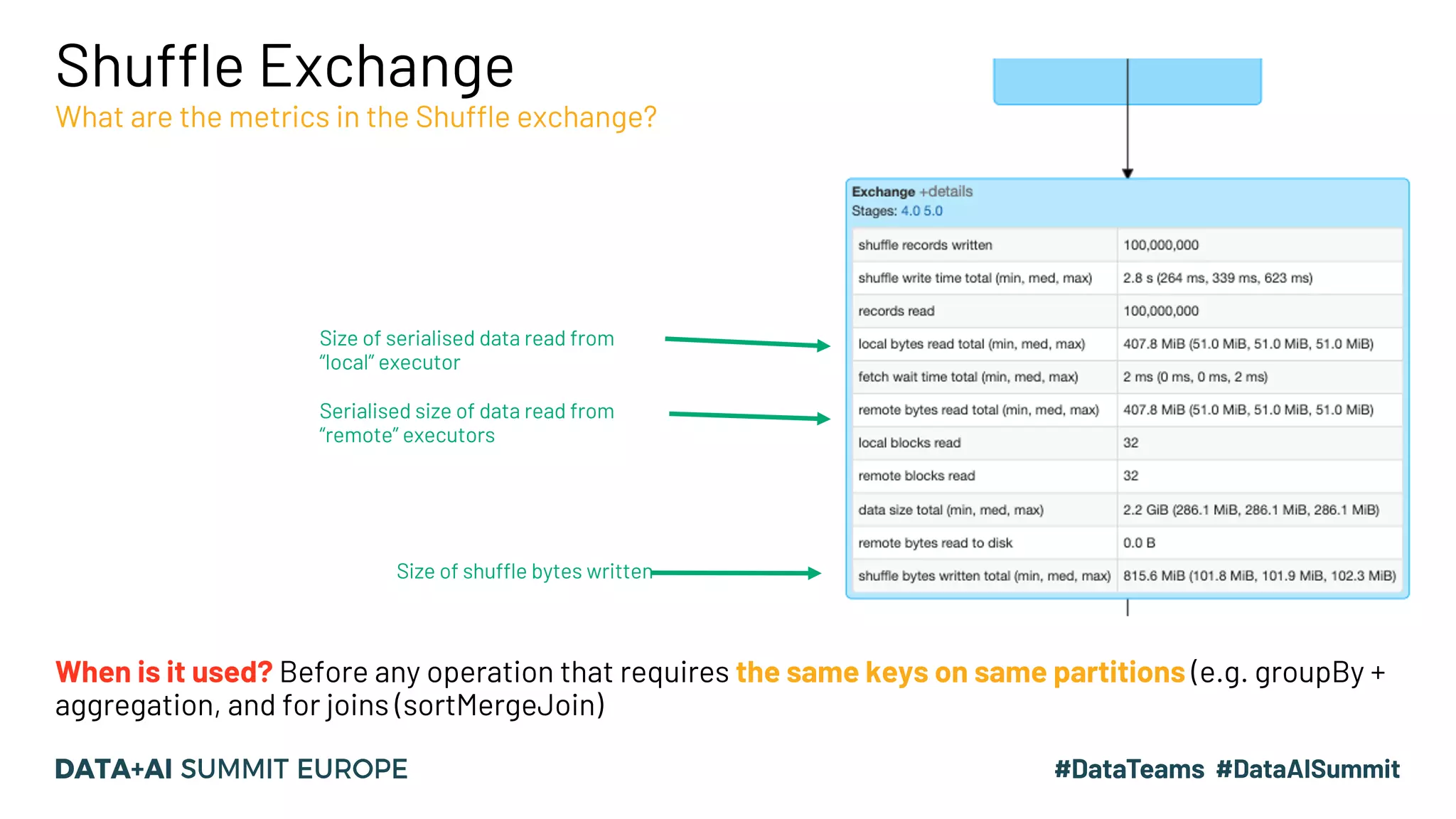
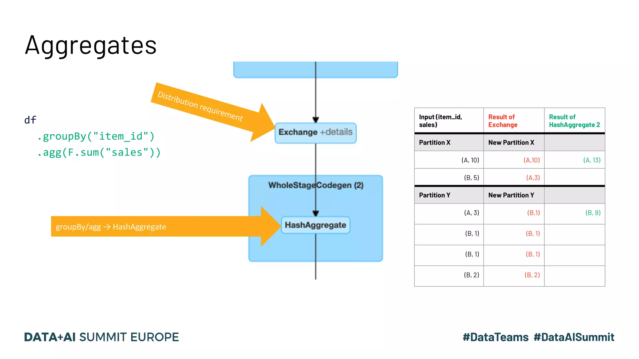
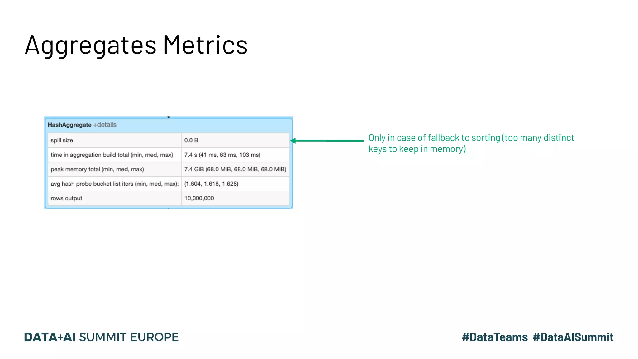
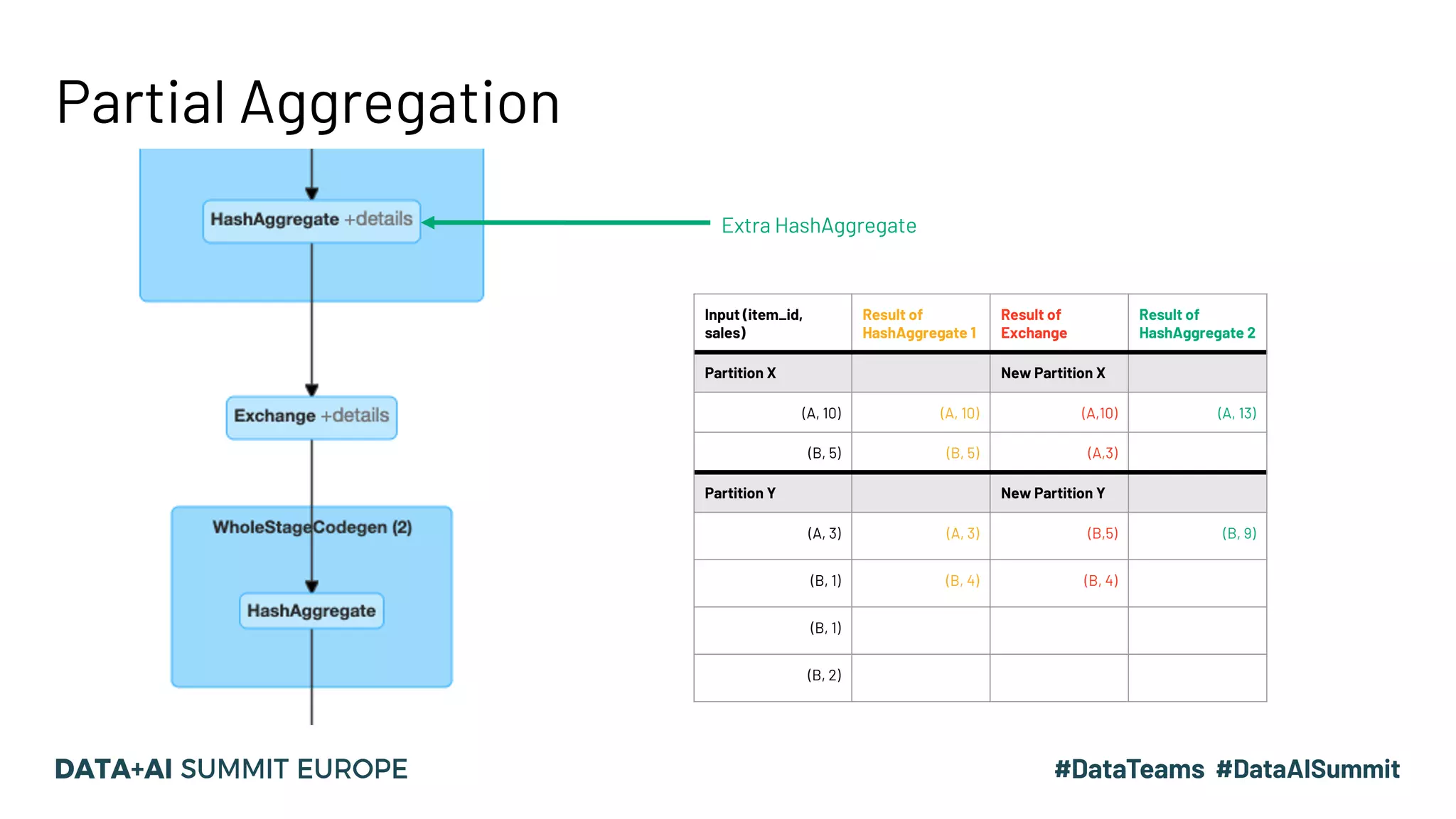
![A simple example (2) # dfSalesSample is some cached dataframe dfItemSales = (dfSalesSample .filter(f.col("item_id") >= 600000) .groupBy("item_id") .agg(f.sum(f.col("sales")).alias("itemSales"))) # Trigger the query dfItemSales.write.format("noop").mode("overwrite").save() == Physical Plan == OverwriteByExpression org.apache.spark.sql.execution.datasources.noop.NoopTable$@dc93aa9, [AlwaysTrue()], org.apache.spark.sql.util.CaseInsensitiveStringMap@1f +- *(2) HashAggregate(keys=[item_id#232L], functions=[finalmerge_sum(merge sum#1247L) AS sum(cast(sales#233 as bigint))#1210L], output=[item_id#232L, itemSales#1211L]) +- Exchange hashpartitioning(item_id#232L, 8), true, [id=#1268] +- *(1) HashAggregate(keys=[item_id#232L], functions=[partial_sum(cast(sales#233 as bigint)) AS sum#1247L], output=[item_id#232L, sum#1247L]) +- *(1) Filter (isnotnull(item_id#232L) AND (item_id#232L >= 600000)) +- InMemoryTableScan [item_id#232L, sales#233], [isnotnull(item_id#232L), (item_id#232L >= 600000)]](https://image.slidesharecdn.com/15vanwouwthone-201124190155/75/From-Query-Plan-to-Query-Performance-Supercharging-your-Apache-Spark-Queries-using-the-Spark-UI-SQL-Tab-8-2048.jpg)
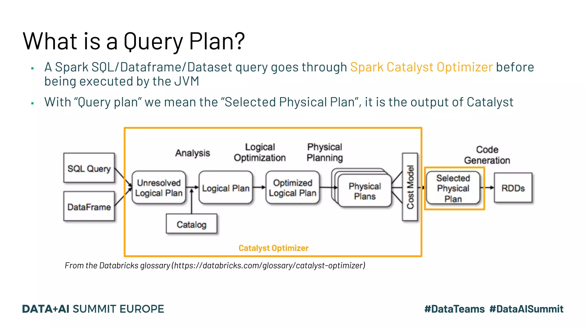
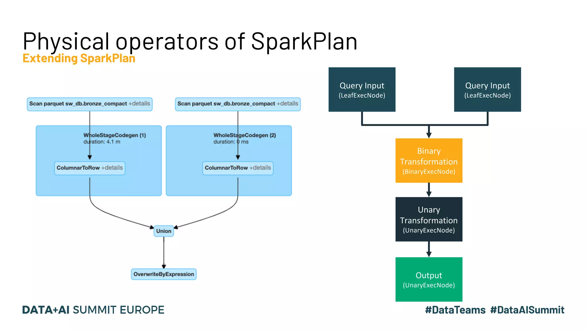
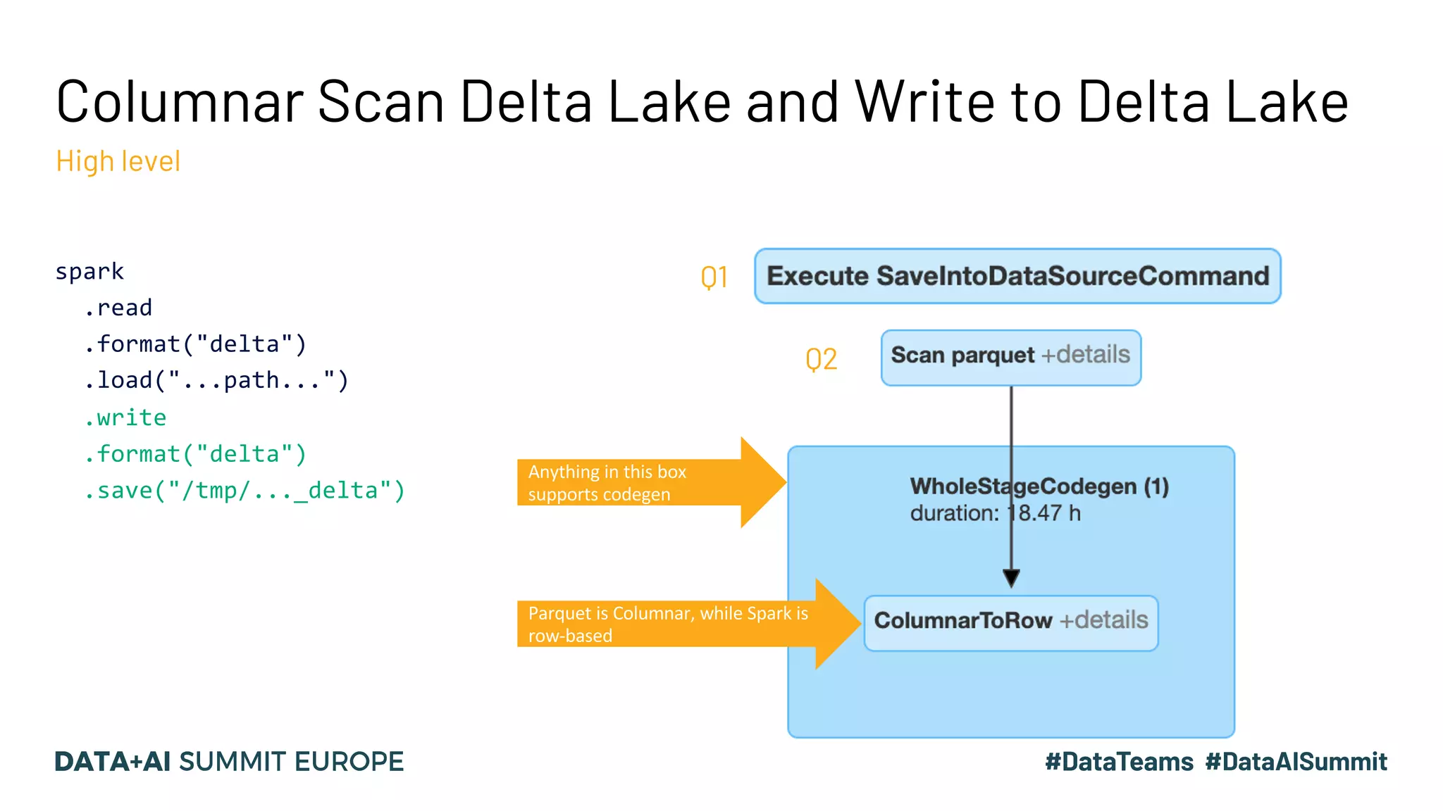
![A simple example (3) == Physical Plan == OverwriteByExpression org.apache.spark.sql.execution.datasources.noop.NoopTable$@dc93aa9, [AlwaysTrue()], org.apache.spark.sql.util.CaseInsensitiveStringMap@1f +- *(2) HashAggregate(keys=[item_id#232L], functions=[finalmerge_sum(merge sum#1247L) AS sum(cast(sales#233 as bigint))#1210L], output=[item_id#232L, itemSales#1211L]) +- Exchange hashpartitioning(item_id#232L, 8), true, [id=#1268] +- *(1) HashAggregate(keys=[item_id#232L], functions=[partial_sum(cast(sales#233 as bigint)) AS sum#1247L], output=[item_id#232L, sum#1247L]) +- *(1) Filter (isnotnull(item_id#232L) AND (item_id#232L >= 600000)) +- InMemoryTableScan [item_id#232L, sales#233], [isnotnull(item_id#232L), (item_id#232L >= 600000)] ▪ What more possible operators exist in Physical plan? ▪ How should we interpret the “details” in the SQL plan? ▪ How can we use above knowledge to optimise our Query?](https://image.slidesharecdn.com/15vanwouwthone-201124190155/75/From-Query-Plan-to-Query-Performance-Supercharging-your-Apache-Spark-Queries-using-the-Spark-UI-SQL-Tab-9-2048.jpg)

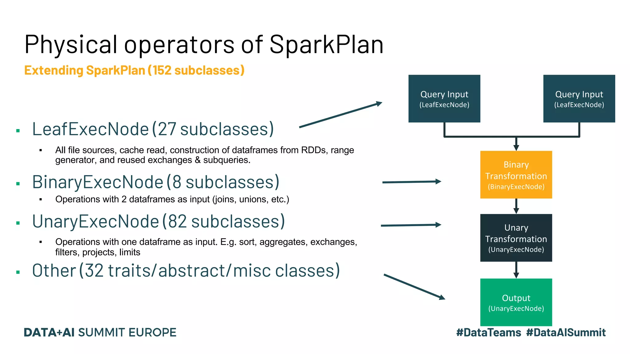

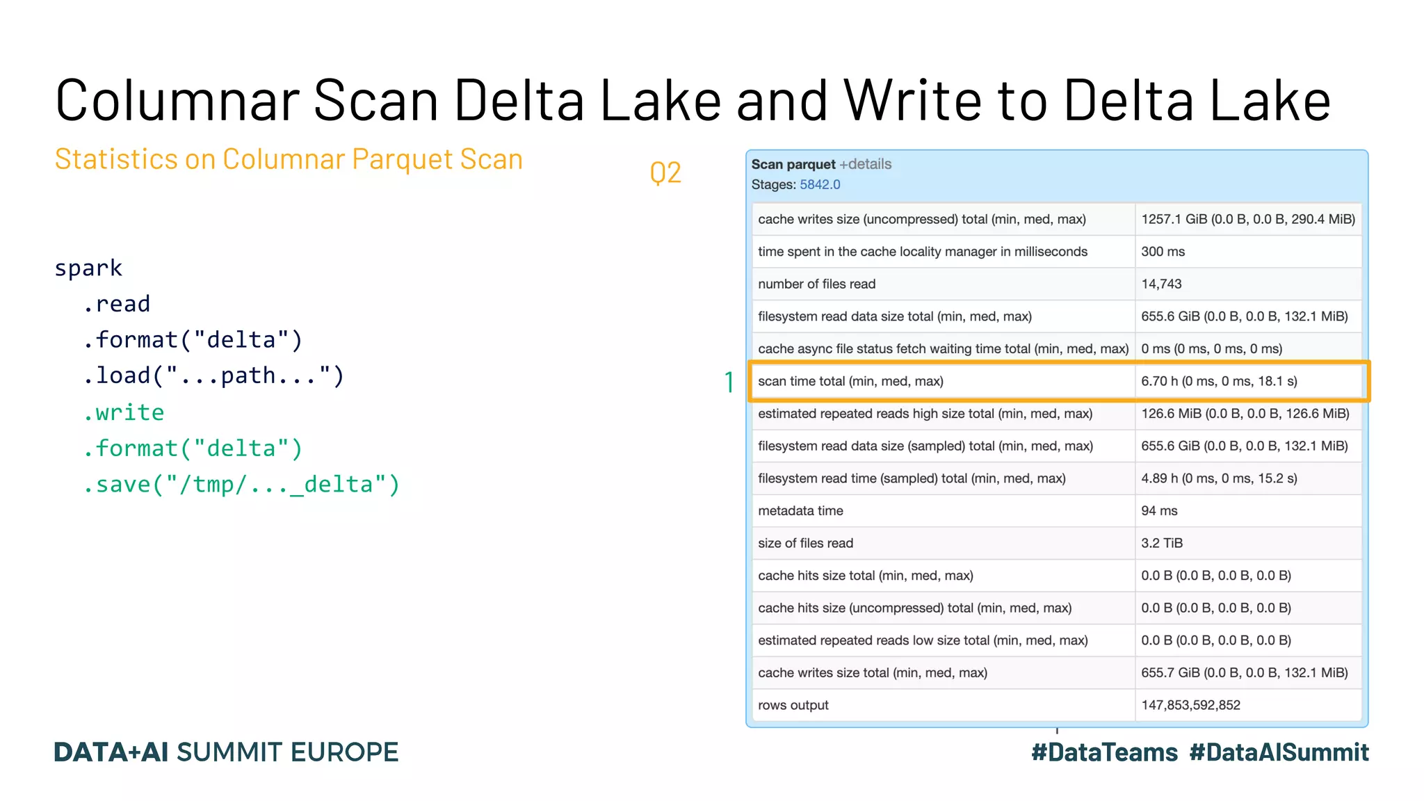


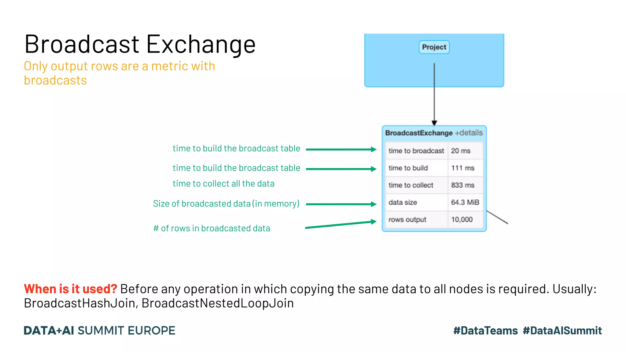


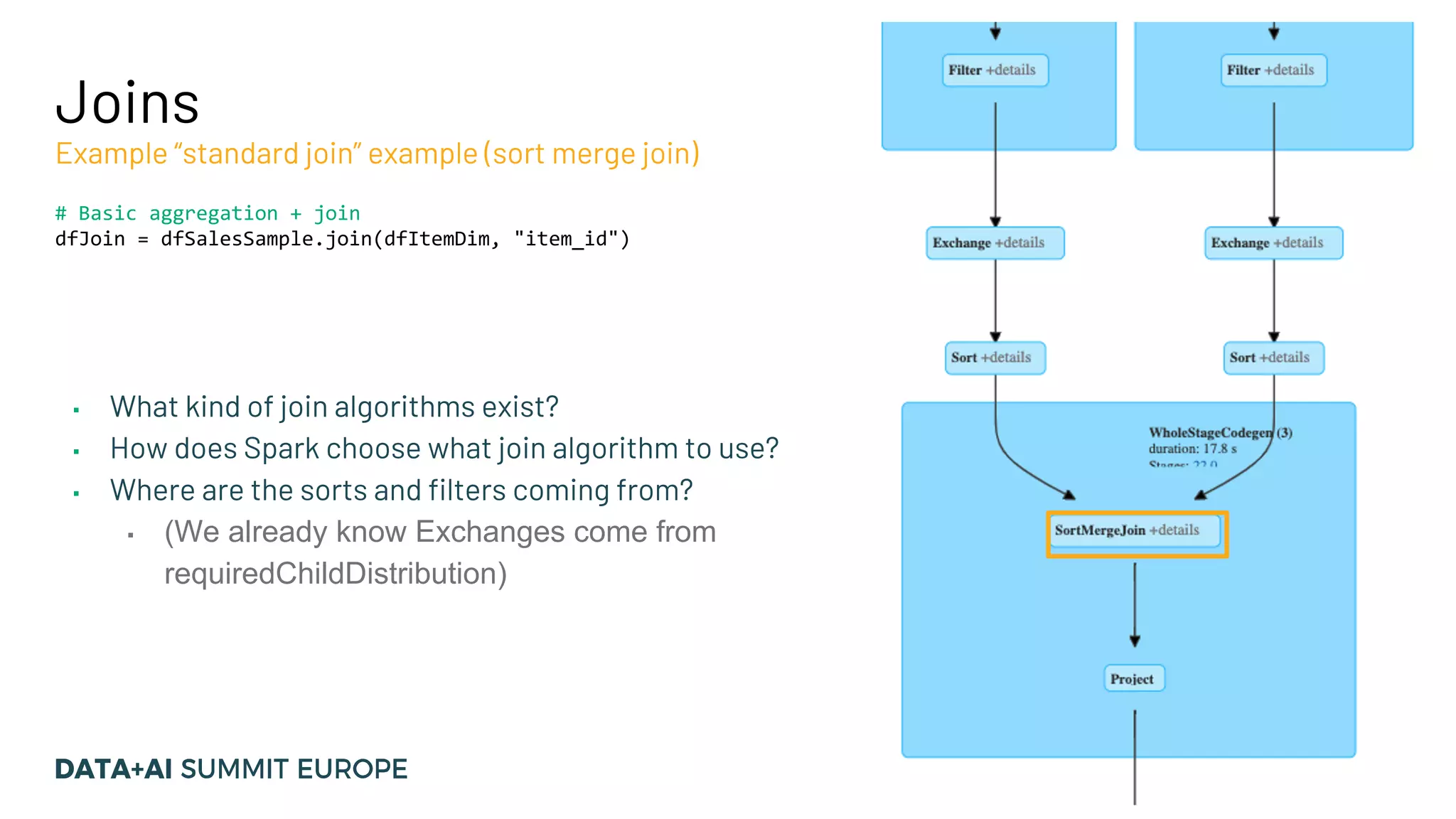
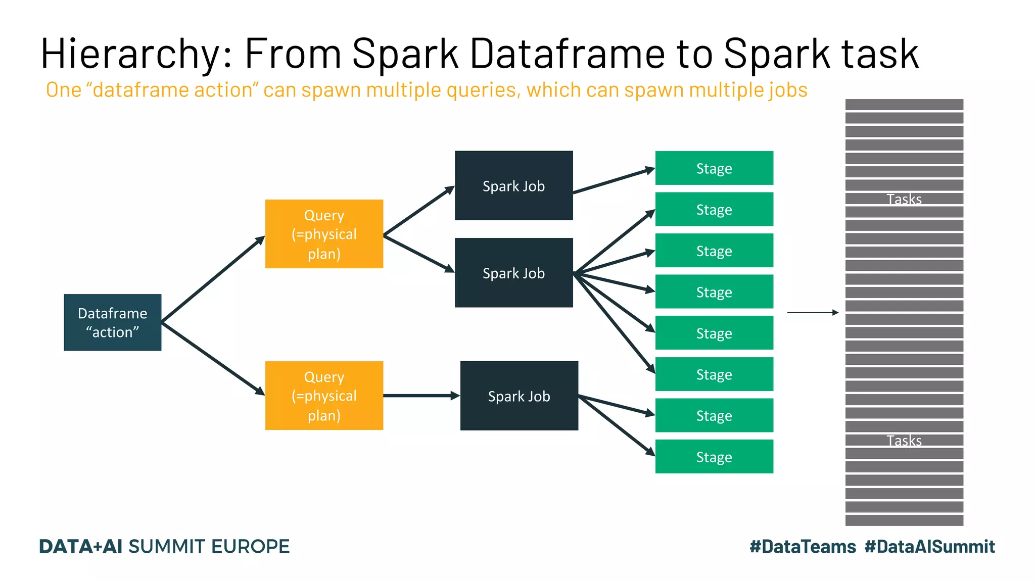
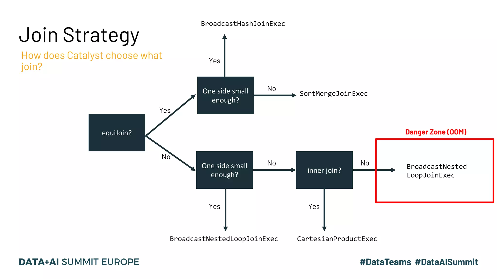
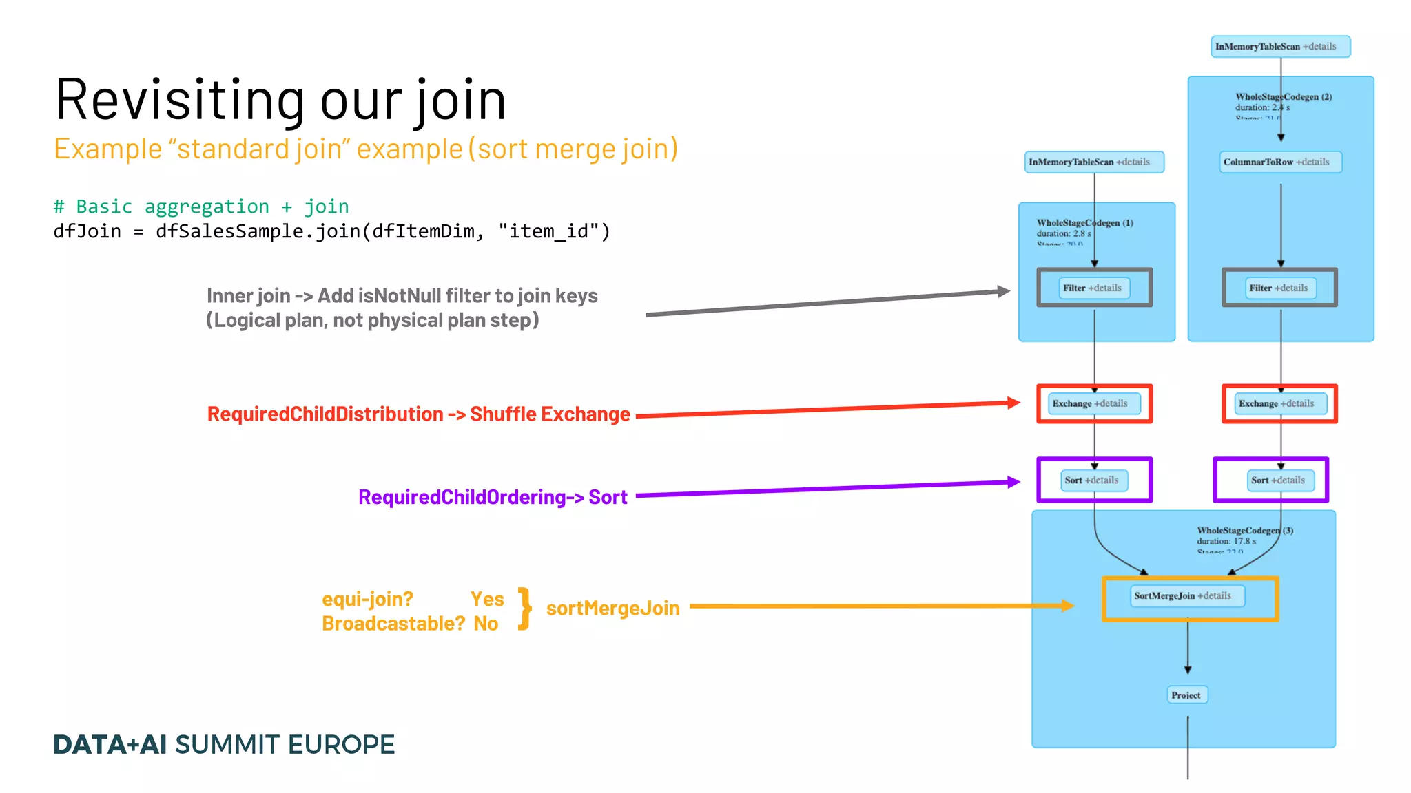
![Join Implementations & Requirements Different joins have different complexities Join Type Required Child Distribution Required Child Ordering Description Complexity (ballpark) BroadcastHashJoinExec One Side: BroadcastDistribution Other: UnspecifiedDistribution None Performs local hash join between broadcast side and other side. O(n) SortMergeJoinExec Both Sides: HashClusteredDistribution Both Sides: Ordered (asc) by join keys Compare keys of sorted data sets and merges if match. O(nlogn) BroadcastNestedLoopJoinExec One Side: BroadcastDistribution Other: UnspecifiedDistribution None For each row of [Left/Right] dataset, compare all rows of [Left/Right] data set. O(n * m), small m CartesianProductExec None None Cartesian product/”cross join” + filter O(n* m), bigger m](https://image.slidesharecdn.com/15vanwouwthone-201124190155/75/From-Query-Plan-to-Query-Performance-Supercharging-your-Apache-Spark-Queries-using-the-Spark-UI-SQL-Tab-39-2048.jpg)
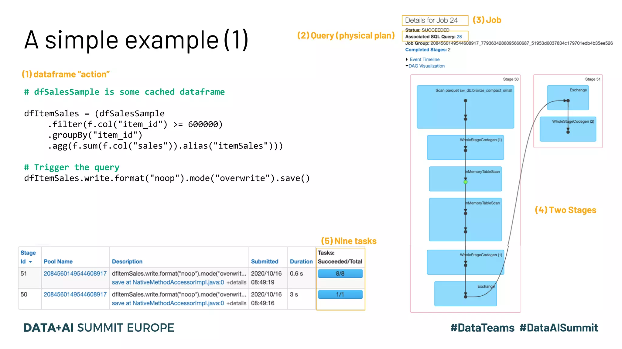
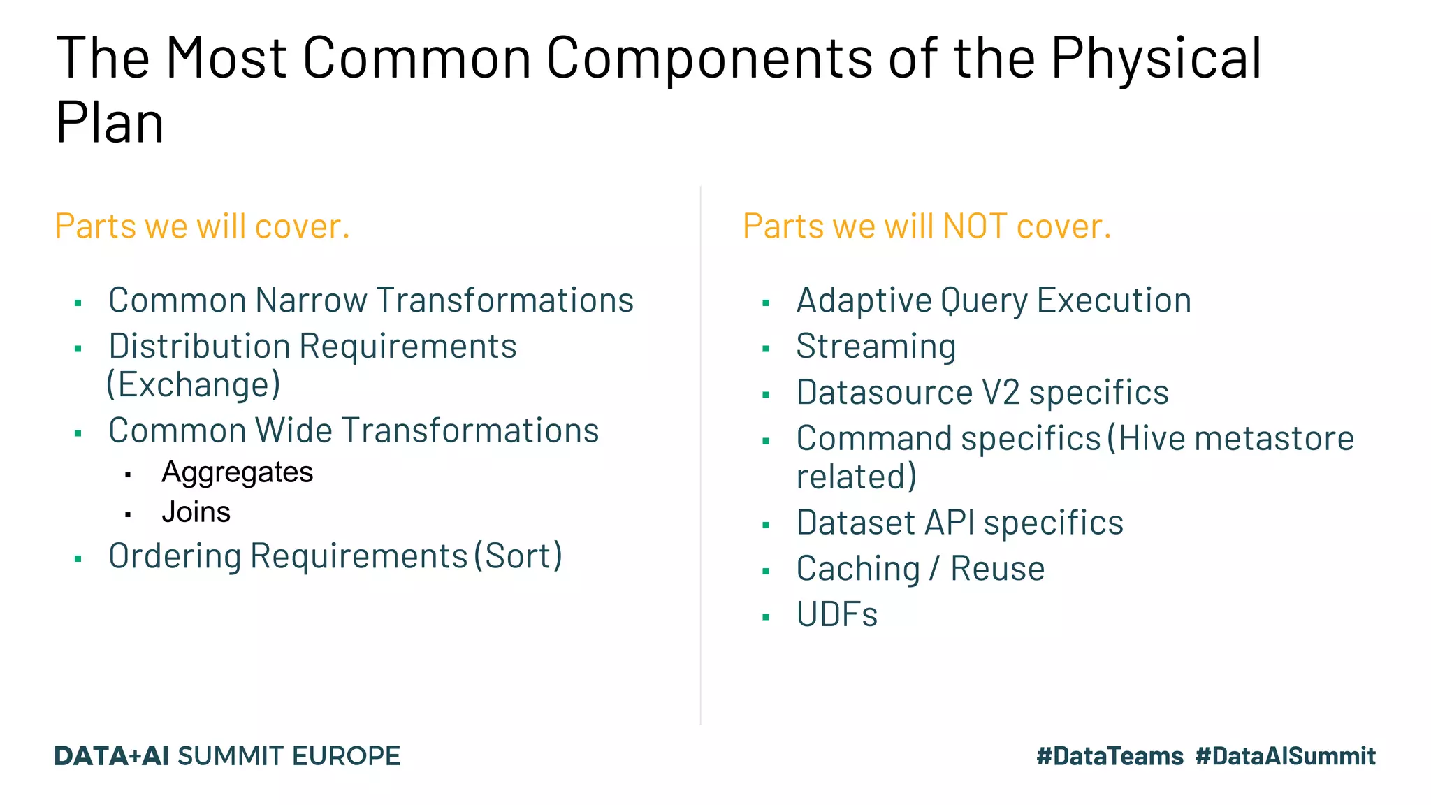
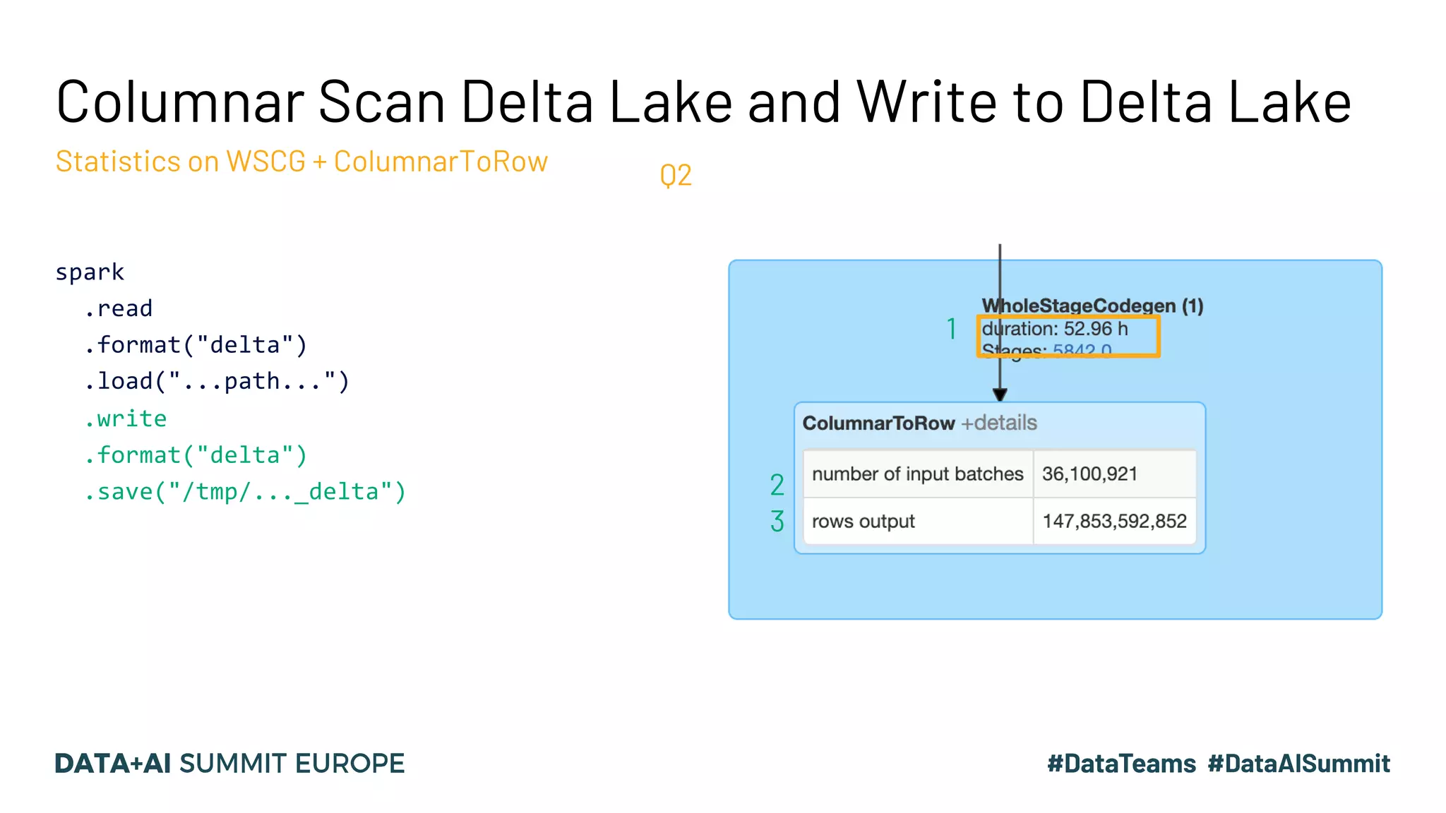
![Ordering requirements Example for SortMergeJoinExec SortMergeJoin (left.id=right.id , Inner) outputOrdering = [left.id, right.id] ASC Sort ([left.id], ASC) SortMergeJoin (left.id=right.id , Inner) requiredChildOrdering = [left.id, right.id] (ASC) outputOrdering = depends on join type Ensure the requirements Sort ([right.id], ASC)](https://image.slidesharecdn.com/15vanwouwthone-201124190155/75/From-Query-Plan-to-Query-Performance-Supercharging-your-Apache-Spark-Queries-using-the-Spark-UI-SQL-Tab-41-2048.jpg)

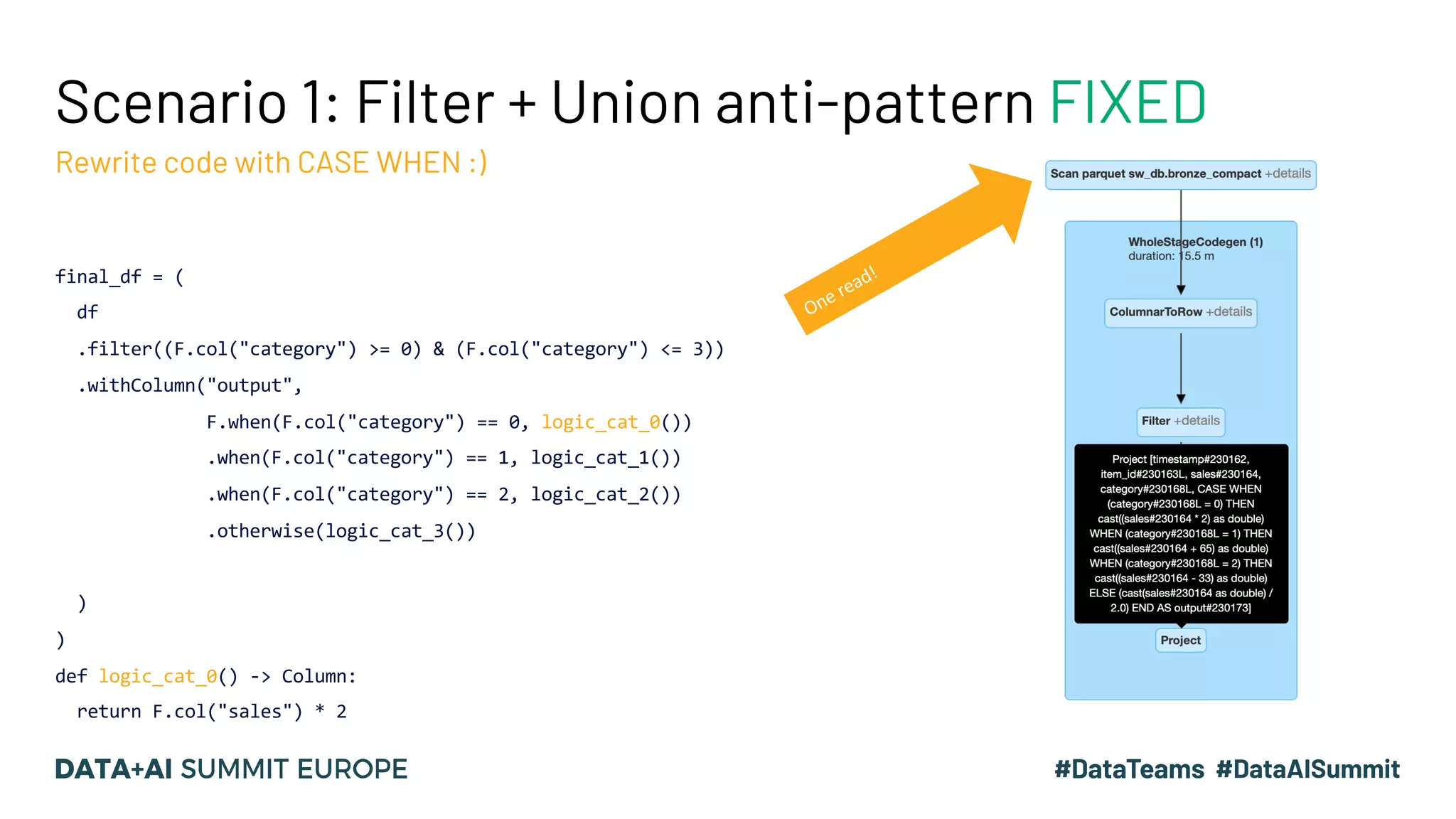
![Scenario 1: Filter + Union anti-pattern E.g. apply different logic based on a category the data belongs to. final_df = functools.reduce(DataFrame.union, [ logic_cat_0(df.filter(F.col("category") == 0)), logic_cat_1(df.filter(F.col("category") == 1)), logic_cat_2(df.filter(F.col("category") == 2)), logic_cat_3(df.filter(F.col("category") == 3)) ] ) … def logic_cat_0(df: DataFrame) -> DataFrame: return df.withColumn("output", F.col("sales") * 2) … Repeated ReadsofData!](https://image.slidesharecdn.com/15vanwouwthone-201124190155/75/From-Query-Plan-to-Query-Performance-Supercharging-your-Apache-Spark-Queries-using-the-Spark-UI-SQL-Tab-44-2048.jpg)
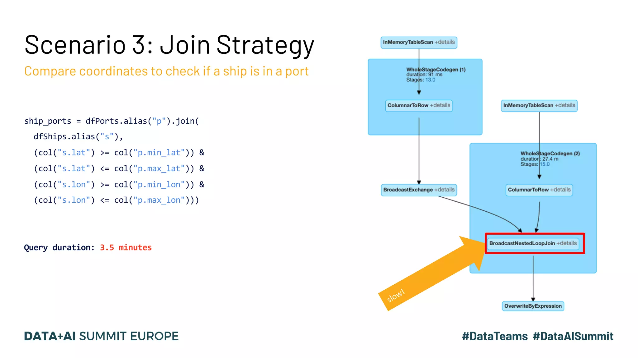
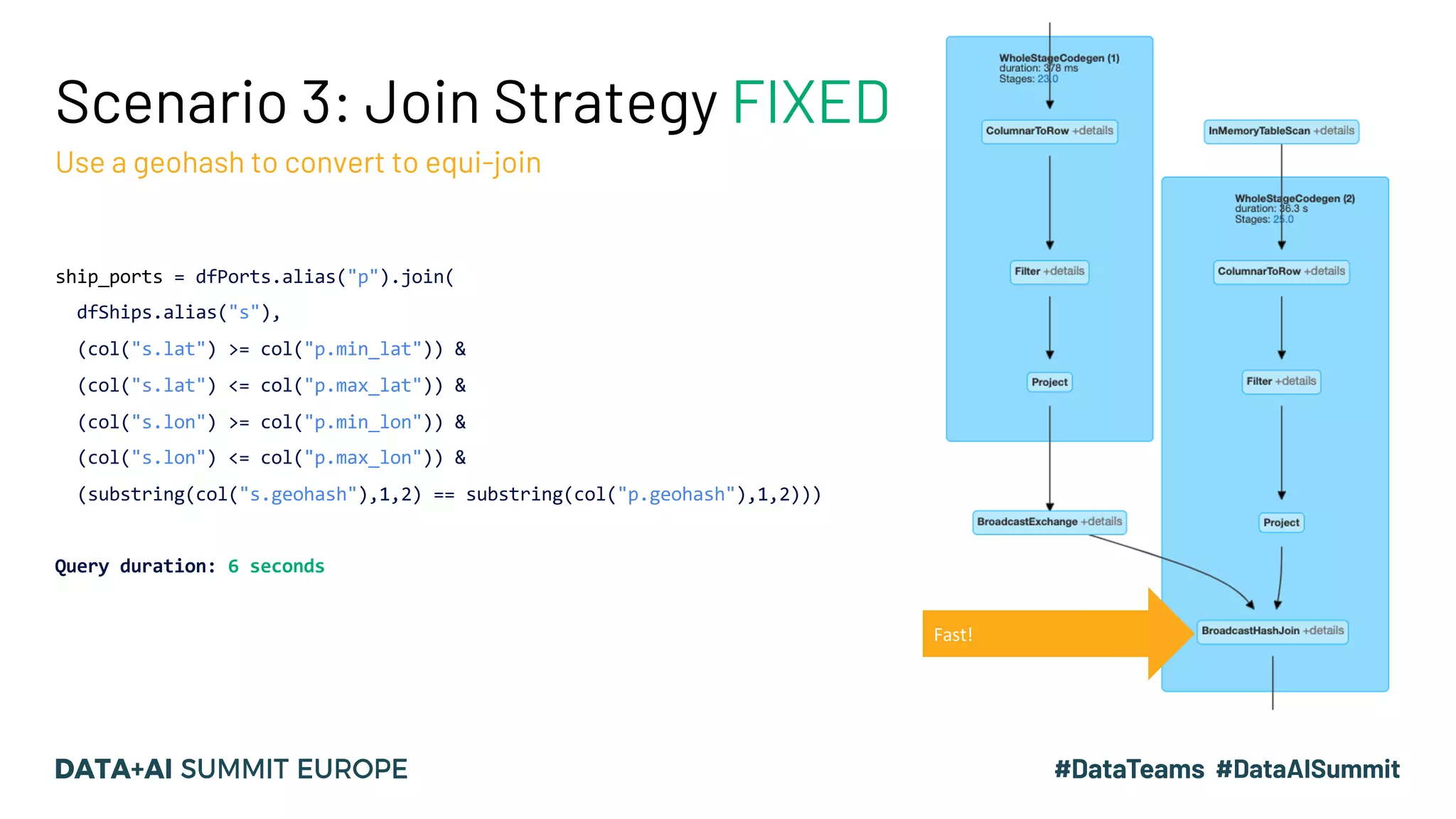


The document discusses optimizing query performance in Apache Spark using the Spark UI SQL tab, which provides insights into query execution and planning through the catalyst optimizer. It outlines the structure of physical plans, common transformation types, and various join strategies to improve query execution efficiency. Several scenarios are provided to illustrate common pitfalls and optimization techniques, such as handling filters, using case statements, and adjusting aggregation strategies.