Consider the following Laplace equation and boundary condition $$\begin{equation}\begin{cases} \Delta \theta(r,\phi)=0 \\ \int d \vec{\ell}\cdot\nabla \theta(r,\phi)=2\pi \end{cases} \end{equation}$$ where $\phi\in[0,2\pi)$, $r\in[0,\infty)$ and the integral is over a circular contour of constant $r$ around the origin such that $d\vec{\ell}=rd\phi \hat{\phi}$ with $\hat{\phi}$ a unit vector in direction $\phi$. The solution to this equation is simply $\theta(r,\phi)=\phi$.
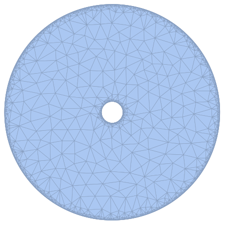
I want to learn how to solve this equation numerically in Mathematica and (approximately) recreate the solution in Cartesian coordinates. To this end, I'm taking a cylindrical domain with an annulus to avoid problems at $r=0$. The outer radius is $R_{1}=1$ and the inner radius is $R_{0}=0.1$. The domain looks like this
Following Solve Laplace equation in Cylindrical - Polar Coordinates, I seem to get the correct solution in polar coordinates but not in Cartesian coordinates and I don't understand why.
Any help is appreciated.
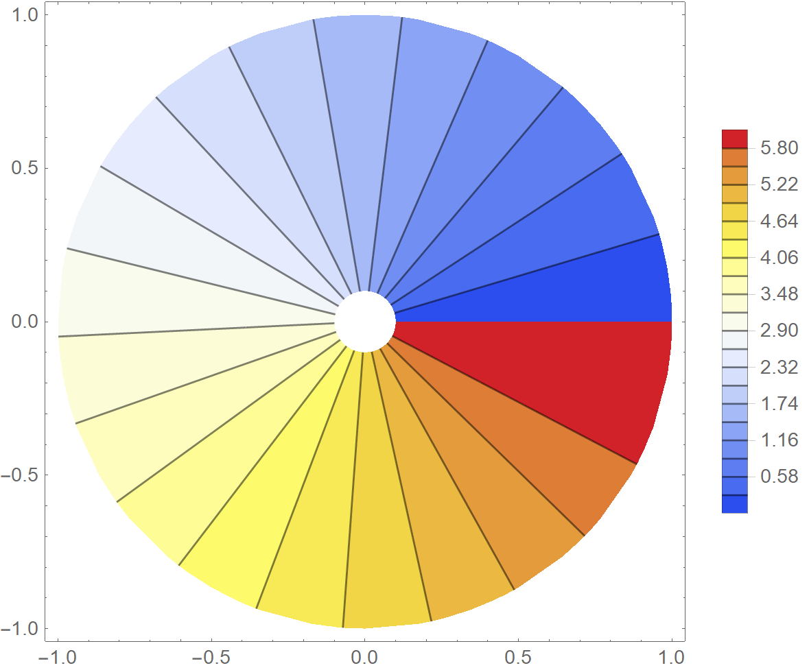
In Polar coordinates I get
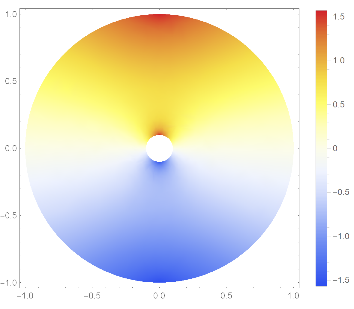
and in Cartesian coordinates I get
This is the code in polar coordinates
R1 = 1; R0 = 0.1; regionCyl = DiscretizeRegion[ RegionDifference[ ImplicitRegion[ 0 <= r <= R1 && 0 <= \[Phi] <= 2 \[Pi], {r, \[Phi]}], ImplicitRegion[ 0 <= r <= R0 && 0 <= \[Phi] <= 2 \[Pi], {r, \[Phi]}]], PrecisionGoal -> 6]; laplacianCil = Laplacian[\[Theta][r, \[Phi]], {r, \[Phi]}, "Polar"]; boundaryConditionCil = {DirichletCondition[\[Theta][ r, \[Phi]] == \[Phi], {r == R0, 0 <= \[Phi] <= 2 \[Pi]}], DirichletCondition[\[Theta][r, \[Phi]] == \[Phi], {r == R1, 0 <= \[Phi] <= 2 \[Pi]}]}; solCyl = NDSolveValue[{laplacianCil == 0, boundaryConditionCil}, \[Theta], {r, \[Phi]} \[Element] regionCyl, MaxSteps -> Infinity]; potentialSquareRepresentation = ContourPlot[ solCyl[r, \[Phi]], {r, \[Phi]} \[Element] solCyl["ElementMesh"], ColorFunction -> "Temperature", Contours -> 20, PlotLegends -> Automatic]; potentialCylindricalRepresentation = Show[potentialSquareRepresentation /. GraphicsComplex[array1_, rest___] :> GraphicsComplex[(#[[1]] {Cos[#[[2]]], Sin[#[[2]]]}) & /@ array1, rest], PlotRange -> Automatic] and this is the code in Cartesian coordinates
R1 = 1; R0 = 0.1; regionCyl = DiscretizeRegion[ RegionDifference[ImplicitRegion[Sqrt[x^2 + y^2] <= R1, {x, y}], ImplicitRegion[Sqrt[x^2 + y^2] <= R0, {x, y}]], PrecisionGoal -> 7]; laplacian = Laplacian[\[Theta][x, y], {x, y}]; boundaryCondition = {DirichletCondition[\[Theta][x, y] == ArcSin[y/Sqrt[x^2 + y^2]], {Sqrt[x^2 + y^2] == R0, 0 <= y/Sqrt[x^2 + y^2] <= 2 \[Pi]}], DirichletCondition[\[Theta][x, y] == ArcSin[y/Sqrt[x^2 + y^2]], {Sqrt[x^2 + y^2] == R1, 0 <= y/Sqrt[x^2 + y^2] <= 2 \[Pi]}]}; sol = NDSolveValue[{laplacian == 0, boundaryCondition}, \[Theta], {x, y} \[Element] regionCyl, MaxSteps -> Infinity]; DensityPlot[sol[x, y], {x, y} \[Element] regionCyl, ColorFunction -> "TemperatureMap", PlotLegends -> Automatic, ImageSize -> Medium] 
NDSolveValuebeing incorrect (I haven't checked but it lookes plausible to me.) The problem is that the pde you gave cannot be interpreted as a pde on the annulus: The boundary condition forbids that. In fact, $(r,\varphi) \mapsto \varphi$ is not a harmonic function on the annulus, in particular, because it must have a jump. $\endgroup$