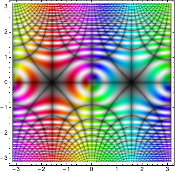
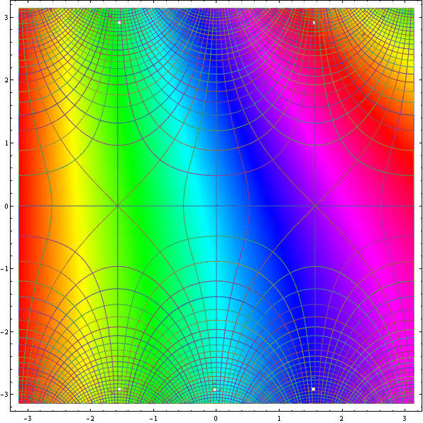
I already mentioned Bernd Thaller's package Graphics`ComplexPlot` in the comments; if one blends the ideas from Artes's and Heike's answers, and then use the function $ComplexToColorMap[] from Thaller's package (I won't include it here; again, see the package for that), we get this:
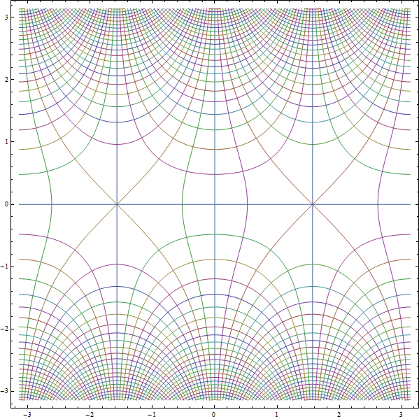
Needs["Graphics`ComplexPlot`"] (* Thaller's package; get it yourself *) f1 = RegionPlot[True, {x, -Pi, Pi}, {y, -Pi, Pi}, ColorFunction -> ($ComplexToColorMap[Abs[Sin[#1 + I #2]], Arg[Sin[#1 + I #2]], {Pi, 1/10, 1, 1/10, 1}] &), ColorFunctionScaling -> False, PlotPoints -> 200]; f2 = ContourPlot[ Evaluate@{Table[Re@Sin[x + I y] == 1/2 k, {k, -25, 25}], Table[Im@Sin[x + I y] == 1/2 k, {k, -25, 25}]}, {x, -Pi, Pi}, {y, -Pi, Pi}, PlotPoints -> 100, ContourStyle -> Gray]; f3 = ContourPlot[ Evaluate@Table[Abs@Sin[x + I y] == 1/2 k, {k, -25, 25}], {x, -Pi, Pi}, {y, -Pi, Pi}, PlotPoints -> 100, ContourStyle -> White, MaxRecursion -> 5]; Show[f1, f2, f3]
The $ComplexToColorMap[] function could probably be optimized a fair bit for new Mathematica, but I won't get into that for now. One might also consider tweaking the Opacity[] of the contour lines for the absolute value as well, but I'll leave that as an experiment for the reader.
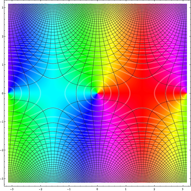
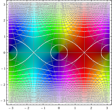
Another thing you can try:
RegionPlot[True, {x, -Pi, Pi}, {y, -Pi, Pi}, ColorFunction -> ($ComplexToColorMap[Abs[Sin[#1 + I #2]], Arg[Sin[#1 + I #2]], {Pi, 1/50, 1, 1/50, 1}] &), ColorFunctionScaling -> False, Mesh -> 51, MeshFunctions -> {Re[Sin[#1 + I #2]] &, Im[Sin[#1 + I #2]] &}, MeshStyle -> Gray, PlotPoints -> 95]