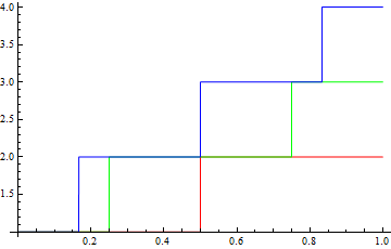
Usually, when I plot multiple curves in Mathematica
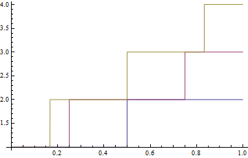
Plot[{x,x^2,x^3},{x,0,1}] they are given different colors. However, if I try to construct a list inside the Plot[] function,
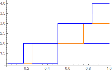
Plot[Table[x^n, {n, 1, 3}], {x, 0, 1}] this doesn't work and all the curves come out the same color. The standard advice (e.g. here, here and here), which works but which I don't fully understand, is to wrap the Table[] with an Evaluate[]:
Plot[Evaluate[Table[x^n, {n, 1, 3}]], {x, 0, 1}] or equivalently
f[x_,n_]:=x^n; Plot[Evaluate[Table[f[x,n], {n, 1, 3}]], {x, 0, 1}] This work in this case, because f[x_]:=x^n is a simple function. However, suppose I have a complicated function g[y] which uses its argument y as a bound for an iterator:
g[y_] := Total[Table[1, {z, 1, Round[y + 1]}]] Mathematica is not smart enough to recognize that this is equivalent to g[y_]:=Round[y]+1, and usually such a simplification will not be possible anyways. g[y] cannot be evaluated symbolically, because of the iterator, although it's still plenty fast when given a machine number. Then trying to plot various curves using a table constructed with g[y] without Evaluate[]
Plot[Table[g[x*n], {n, 1, 3}], {x, 0, 1}] will make all the curves the same color. Adding Evaluate[]
Plot[Evaluate[Table[g[x*n], {n, 1, 3}]], {x, 0, 1}] causes Mathematica to throw an error message about using a bad iterator. (Table::iterb: "Iterator {z,1,Round[1+x]} does not have appropriate bounds).
Why, exactly, is Evaluate[] necessary in the simple case? Is it true that Plot[] is interpreting the table as a multi-valued function? Why?
How can we achieve the same result in the complicated case where the technique fails?