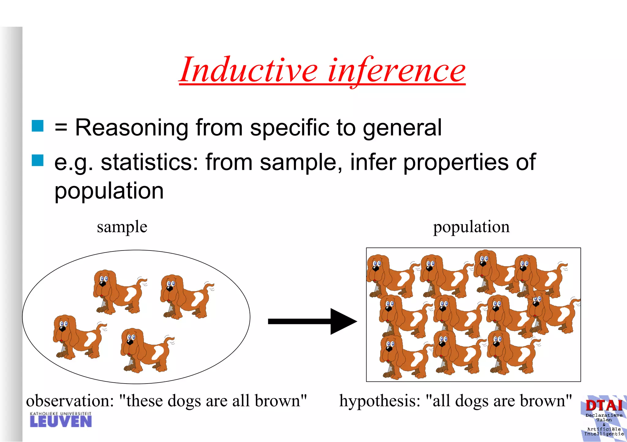
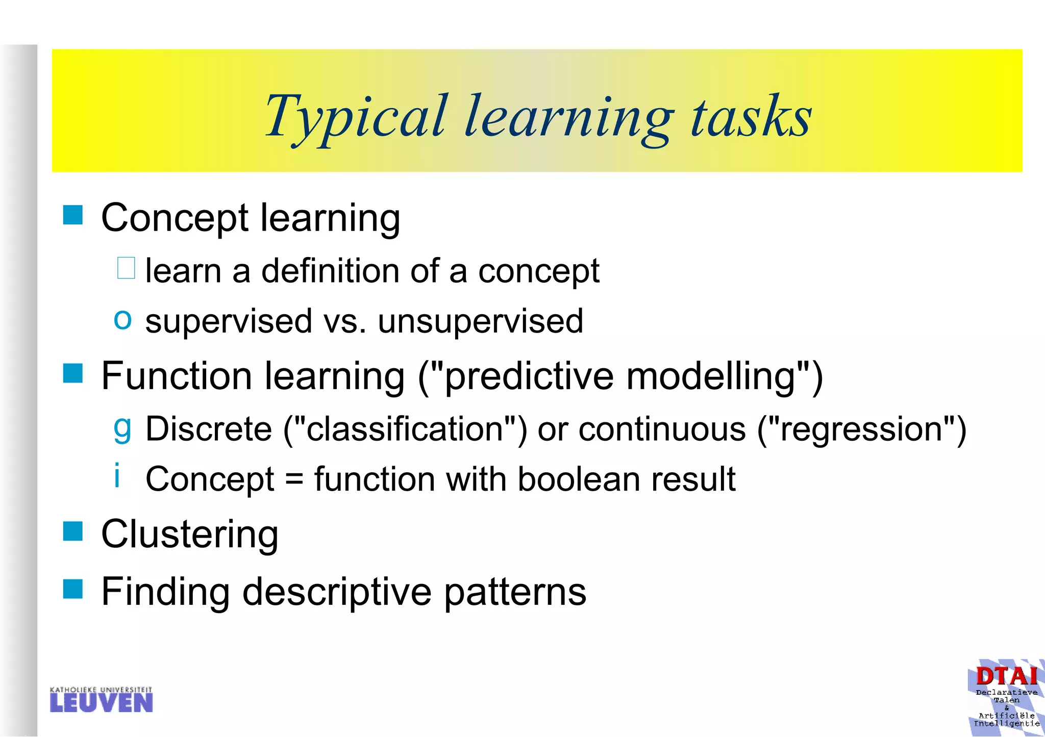
This document provides an introduction to machine learning and inductive inference. It discusses what machine learning is, common learning tasks like concept learning and function learning, different data representations, and example applications such as knowledge discovery and building adaptive systems. The course will cover generalizing from specific examples to broader concepts through inductive inference and different learning approaches.
![How to obtaining training examples? we need a set of examples [bp, rp, bk, rk, bt, rt, V] bp etc. easy to determine; but how to guess V? we have indirect evidence only! possible method: with V(s) true target function, V’(s) learnt function, V t (s) training value for a state s: V t (s) <- V’(successor(s)) adapt V’ using V t values (making V’ and V t converge) hope that V’ will converge to V intuitively: V for end states is known; propagate V values from later states to earlier states in the game](https://image.slidesharecdn.com/machine-learning-and-inductive-inference3031/75/Machine-Learning-and-Inductive-Inference-19-2048.jpg)

![Example decision tree 2 Again from Mitchell: tree for predicting whether C-section necessary Leaves are not pure here; ratio pos/neg is given Fetal_Presentation Previous_Csection + - - 1 2 3 0 1 [3+, 29-] .11+ .89- [8+, 22-] .27+ .73- [55+, 35-] .61+ .39- Primiparous … …](https://image.slidesharecdn.com/machine-learning-and-inductive-inference3031/75/Machine-Learning-and-Inductive-Inference-66-2048.jpg)
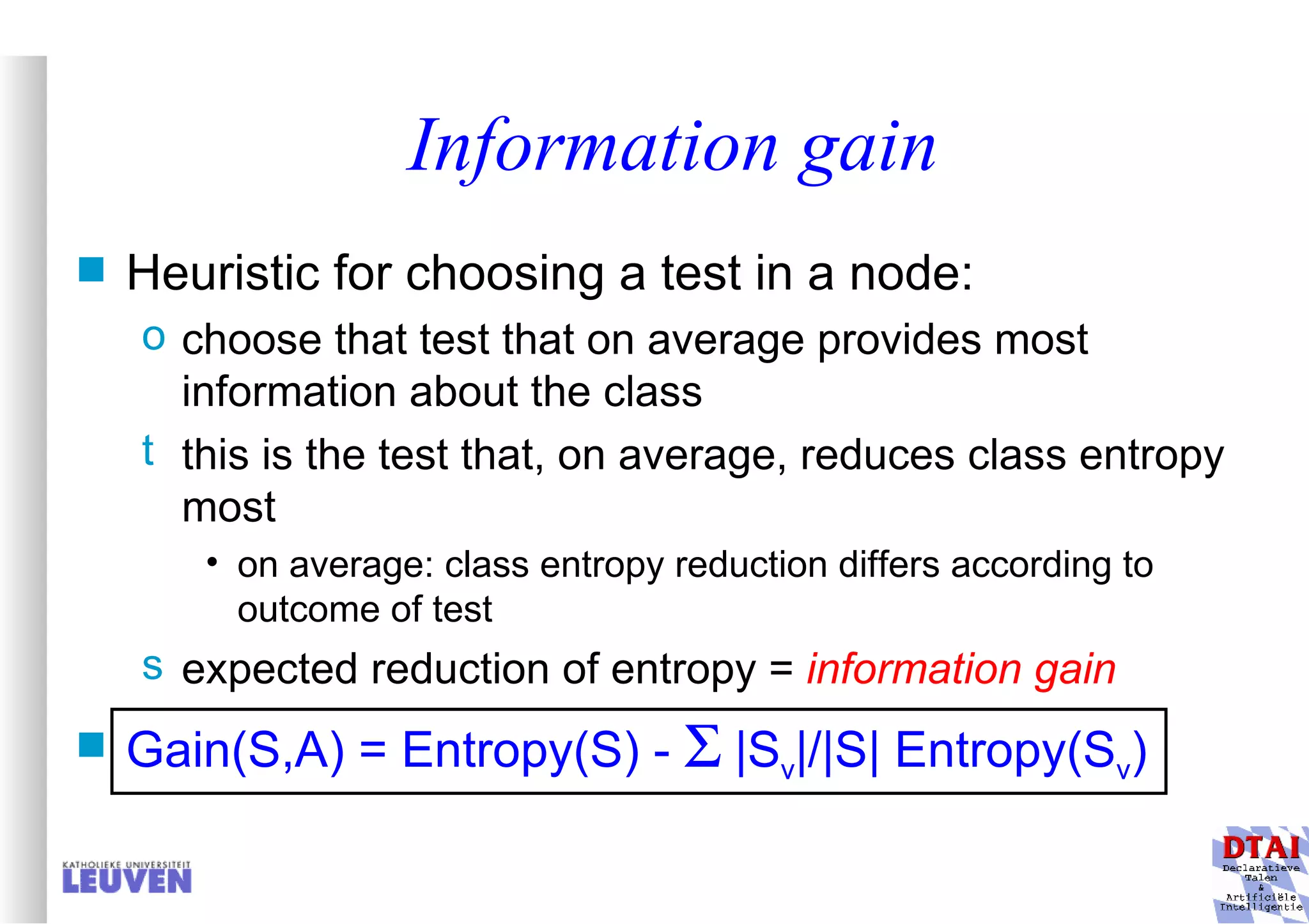
![Example Assume S has 9 + and 5 - examples; partition according to Wind or Humidity attribute Humidity Wind High Normal Strong Weak S: [9+,5-] S: [9+,5-] S: [3+,4-] S: [6+,1-] S: [6+,2-] S: [3+,3-] E = 0.985 E = 0.592 E = 0.811 E = 1.0 E = 0.940 E = 0.940 Gain(S, Humidity) = .940 - (7/14).985 - (7/14).592 = 0.151 Gain(S, Wind) = .940 - (8/14).811 - (6/14)1.0 = 0.048](https://image.slidesharecdn.com/machine-learning-and-inductive-inference3031/75/Machine-Learning-and-Inductive-Inference-77-2048.jpg)
![Assume Outlook was chosen: continue partitioning in child nodes Outlook ? ? Yes Sunny Overcast Rainy [9+,5-] [2+,3-] [3+,2-] [4+,0-]](https://image.slidesharecdn.com/machine-learning-and-inductive-inference3031/75/Machine-Learning-and-Inductive-Inference-78-2048.jpg)